The graph shown above summarizes the scans done on two parameters: VFS which has a strong effect on the shape of the output pulse by changing the decay time of the pulse,
and VFP which also affects the shaping but appears to have less of an effect on the output shape.
We are trying to see if using actual collision data, an anzats of signal-to-noise in the system can be found. We are making the assumption that the noise in the detector is well described by the width of pedestals. The choice of signal is obvious; we use a narrow bin of the pedestal subtracted ADC signal per strip. The bin of charge is chosen approximately near the median of the charge distribution.
Most of the collision or pedestal data sets have 5000 events, some of them have twice that many events. The analysis is always done on pedestal subtracted ADCs. The status of all channels is included in the analysis to exclude dead or misbehaving strips. For the first four VFS points we used the strips from quadrant 1 in disc 1. Later, to add more counts to the 
 histograms of interest, I switched to strips from all quadrants in disc 1.
The graph shows that, as expected, the VFS parameter shown with read markers modifies the output shape and producess a clearly visible deterioration of the signal-to-noise performance of the system, (the curve is a spline to guide the eye). Taking some liberties to interpret the red points, one could claim that the the first two points (0, 30) show little change but beyong VFS=60, the signal-to-noise ratio drops. Similar reading can be done on the VFP scan presented in the same figure with blue markers; the effect of this parameter is not so pronounced, but it also shows a flat region up to VFP=60 with a clear drop on the last point. The nominal values we used last year and continue to be in this year configuration files are:       VFP = 30    and VFS = 70.

The magenta star marker shows the result of the same analysis described above but this time the input is a run (14065079) collected with the so called nominal configuration file which had the values VFP=30    and VFS=70. The pedestal file used for this case was extracted from run 14065115. The resulting value of the signal-to-noise ratio sits close to the spline joining the previous VFS measurements. Earlier versions of this blog had a point obtained from an earlier run which did not follow the trend of the scan. Akio was not done with his work on changing clock phases yet.

Out of this first look at the APV parameter scan I would try to build an argument to leave VFP at the value it has now (30) but to lower the value of VFS to a new value closer to 30.

The argument will lean on the fact that as VFS grows the rise time of the pulses gets, in average, slower and has more jitter as can be seen in the acompanying  sets of plots shown below for each value of the VFS parameter. Among other plots, the lower left plot shows the resulting Landau distribution obtained in fitting the selected data pulses. The Landau distribution is plotted at a fixed time value (5) and has the amplitude set to 1. The mean value and the jitter of the rise time for a cut in amplitude:[0.075, 0.09] is shown on the right plot a the accompaning text.
Lowering the value of VFS below 60 would give narrower pulses wich is something we actually should do for high luminosity data collection. At lower values of VFS the pulses have a decently faster rise which in turn helps if we only read 6 or 7 time bins.

-----------------------------------------------------------------------------------------------------------------------------
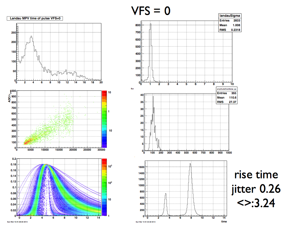
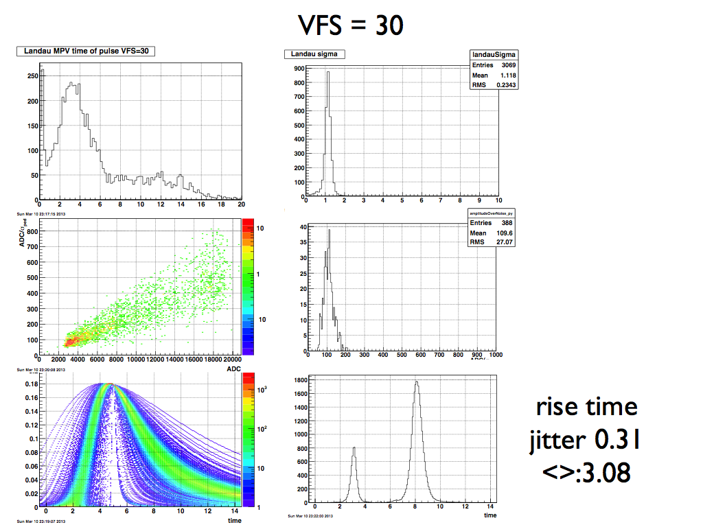
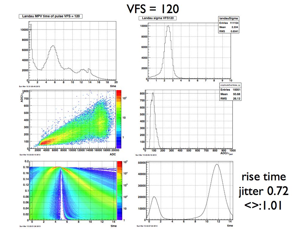
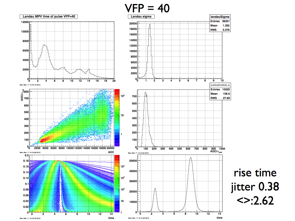
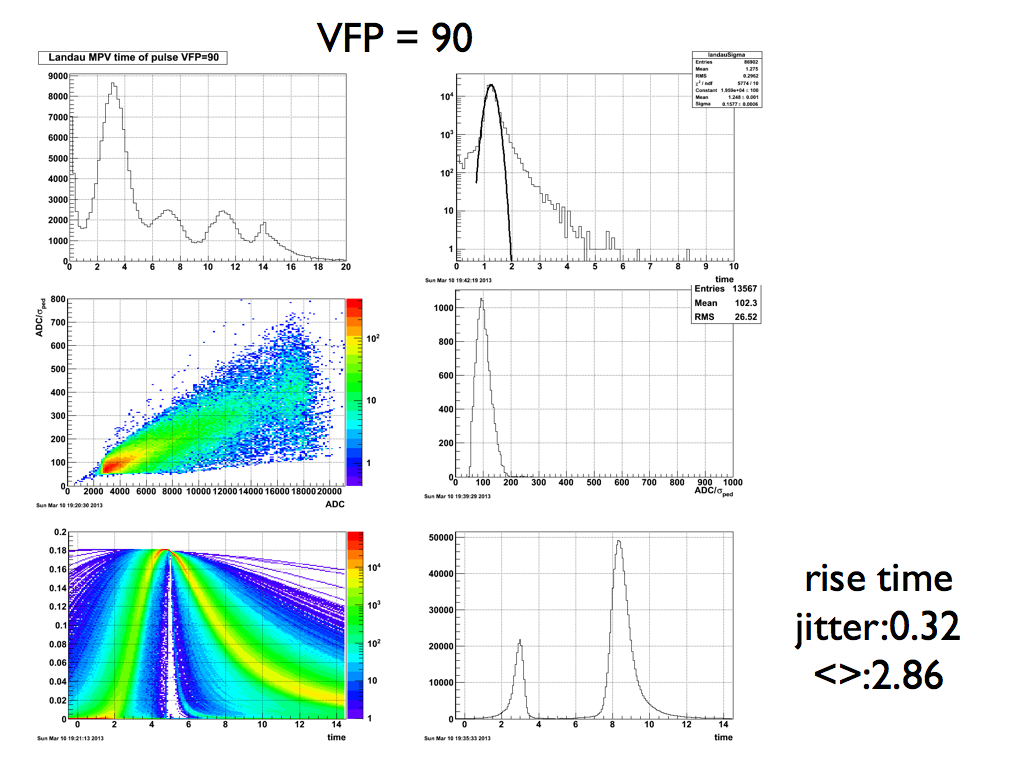
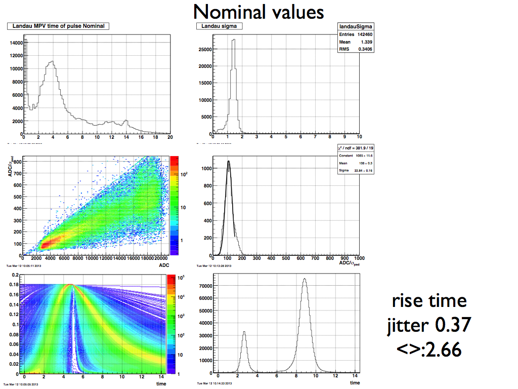
The sets of plots that follow should give an overview of the effect of the relevant parameter change.
The top left plot shows the time of the Landau distribution Most Probable Value (MPV). For the collision data we collected so far, each strip "scope trace" graph shows tails of pulses from earlier bunch crossing. The fit to Landau distributions would then produce MPV low values. Pulses from the bunch crossing just after the one we triggered, are fit with shapes that have high MPV values. To select pulses in time with the triggered collisions I put a cut on the MPV value: [2.5, 6.] The data with VFS=120 is the only case where that cut moves to [3,8].
Pulses that have MPV values within that window and a minimum integrated charge of 50 (amplitude of the Landau fit) are then used for further analysis. The top right plot shows the "sigma" (RMS) value of the Landau shape (this width is a mix of rise and decay times which I do not make an attempt to disentangle).
The middle left plot shows the correlation of signal-to-noise (as ADC divided by pedestal width for each strip used in this analysis) to the actual ADC value (integrated charge in the strip over 15 time bins). The middle right plot shows the projection of the left plot over the y axis for a bin of ADC values [3685, 4439]. The mean value of this distribution together to its associated error is plotted in the first figure of this report.
The bottom left figure has all the fitted Landau shapes drawn at fixed t=5 and amplitude set to 1. The information that can be extracted from this plot (which follow similar plots found in Maxence's thesis (www.google.com/url) may include the average shape for different parameter values, the jitter in rise and fall times which must be a combination of the different strip capacitances and actual jitter in the readout system. The bottom right figure shows a projection of the left figure over the x axis for a narrow window of amplitud [0.075, 0.09]. The left peak show the rising side of the pulses and the right one corresponds to the falling side.

===========================================================================================
VFS = 0

===========================================================================================
VFS = 30

===========================================================================================
vfs = 60

===========================================================================================

VFS = 90

===========================================================================================
VFS = 120

===========================================================================================

===========================================================================================
VFP = 20

===========================================================================================
VFP = 40

===========================================================================================

VFP = 60

===========================================================================================

VFP = 90

10K collision events events written to run14064027 with pedestal collected with the same configuration file in run14063105 

===============================================================================================
===============================================================================================

Nominal values VFS+70 VFP=30