Continuing from drupal.star.bnl.gov/STAR/blog/rjreed/centrality-epd-take-3

These are from UrQMD data, 19.6 GeV, using the fast simulator for the epd written by Mike as detailed above.

The question is, why does the linear weight do so poorly?  First lets bring some relevant plots from the blog above.

Figure 1: Forward Charged Particle Multiplicity (2.1 < |eta| < 5.1) - Left shows the 2D correlation with the impact parameter (b), the middle plot shows the b distribution for selection cuts on particle multiplicity, the right shows the particle multiplicity distribution with the centrality cuts.

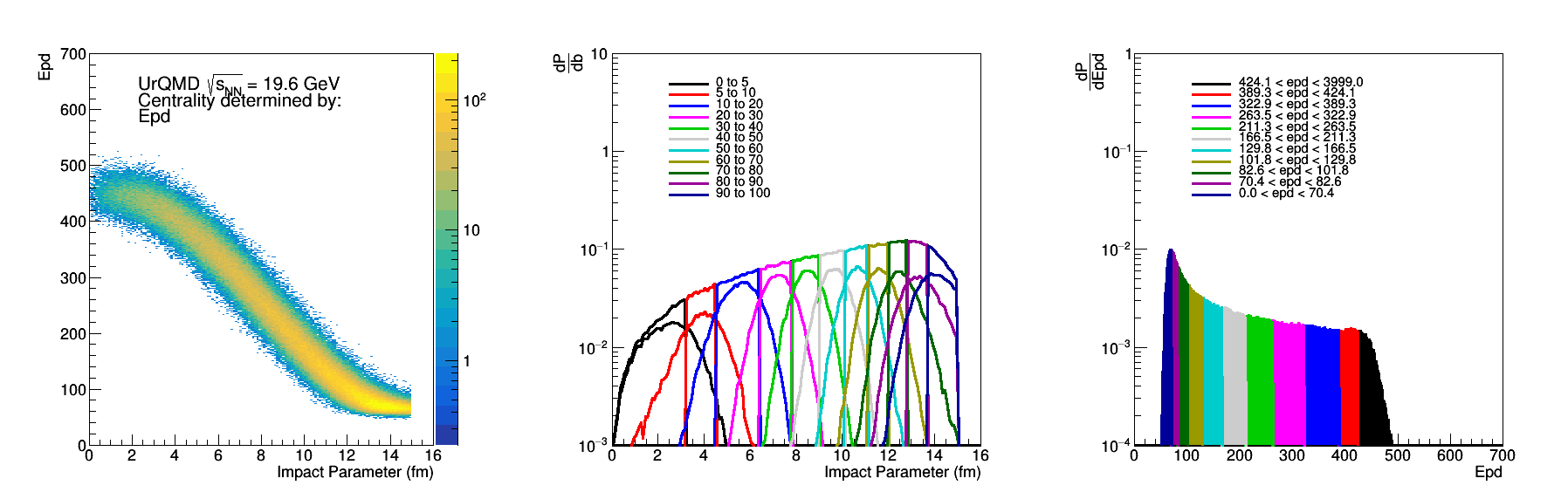
Figure 2: Epd Nmip sum, where 0.2 < Nmip < 2, if Nmip> 2 then Nmip=2.  Similar distributions as above.

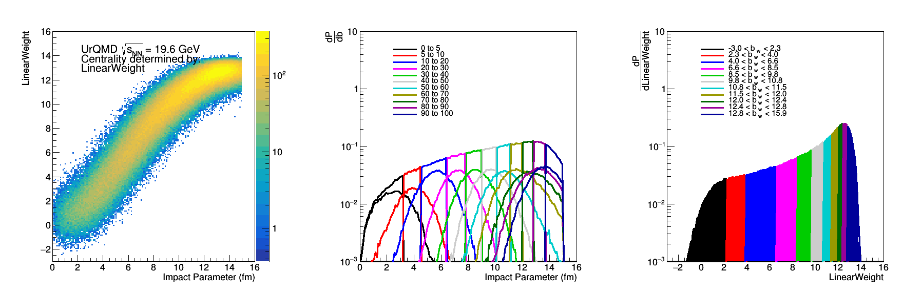
Figure 3: Linear Weight of the epd Mips shown in figure 2.

Figure 4:  Linear weights of the particle counts (separating by EPD rings) of the distributions shown in Figure 1.

Figure 5: Sigma_X^2/Sigma_b^2 with the most central events on the right and the most peripheral on the left.

In Figure 5 there are a few things to be noticed, first of all the discontinuity at the most central end is due to the fact that the first two bins are 5% central bins rather than 10%.  The linear weight scheme did worse for both the particle count and the nmip distributions, so it is not due to the fluctuations.  The linear weight for particle counts did better than the linear weight scenario of the EPD mips, which isn't surprising.  The fact that the epd mip distribution did slightly better than the particle counts is also surprising.

I will focus on the Nmip distributions...  First lets look at the distribution ring by ring.

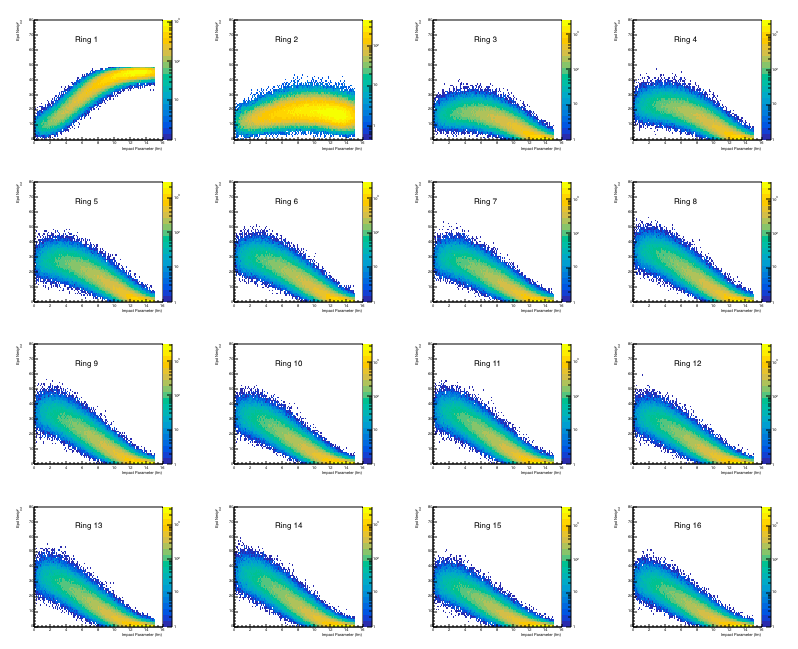
Figure 6: Epd Nmip sum by ring, where 0.2 < Nmip < 2, if Nmip> 2 then Nmip=2.

Figure 7: 1D projections of Figure 8.

We see from Figure 7 and 8 that ring 1 is the only one that saturates for this energy level, and that only rings 1 and 2 don't have a significant 0 population.  The weird "bump" at 2 for the lower level rings corresponds to events where 1 tile had the maximum NMip distribution of 2.

Repeating the weights:
ring      weight
    1    0.273525
    2    0.0296001
    3    -0.0601397
    4    -0.0477917
    5    -0.0337742
    6    -0.0232543
    7    -0.0117203
    8    -0.00703337
    9    -0.0024524
    10    0.00399249
    11    0.00605742
    12    0.00908568
    13    0.00985799
    14    0.0102809
    15    0.013745
    16    0.0136804

We see the strongest weight is given to ring 1.  Looking at these, though, I'm a little surprised because ring 2 doesn't look like it has a strong correlation with impact parameter, but the others do. I'm also a little baffled at the different signs.  Naively I would have expected a positive value for ring 1, a value close to 0 for 2.  Then negative values for the rest.  Perhaps this is in error.  Regardless, the weight is dominated by ring 1.  The switch of the correlation between counts and impact parameter in ring 1 compared to the others must make the resolution in the counting method worse....

Looking at the minimization parameter for ring 1:

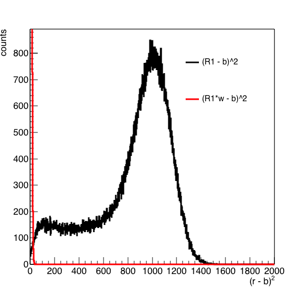
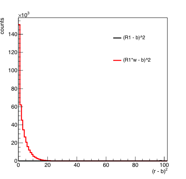
Figure 8: On the left is the distribution of (R1 - b)^2 in black and (R1*w-b)^2 in red.  On the right is a zoomed in version of the distribution.

From figure 8 it seems the minimization routine is doing its job ... moving the large peak at 1000 or so to zero. 

Ok - I think the issue is that the linear weight will ignore the sign of the correlation - the weight itself depends simply on how far the peak of the distribution is from 0.  Basically this weights ring 1 more heavily because more particles hit it in general (at this energy) and thus it needs a larger weight to minimize the distribution.  The average of the impact parameter is 9, so distributions with an average less than 9 will get a negative weight, but can not get a negative weight on the order of the weight of ring 1, just due to the values allowed.  I believe the issue is that the significance of a given ring isn't strictly dependent on how many particles hit it, but how well the number is correlated with b.

So what do use instead?  The covariance of the two axis would be difficult as this depends on the range of the distribution, so I think would suffer the same issues as the linear weight.  Fortunately, root has this convenient normalization routine for TH2 - GetCorrelationFactor() which returns GetCovariance(axis1,axis2)/stddev1/stddev2 - the covariance normalized by the standard deviations of the two distributions.

Ring 1 correlation factor 0.896573
Ring 2 correlation factor 0.0672031
Ring 3 correlation factor -0.824721
Ring 4 correlation factor -0.876886
Ring 5 correlation factor -0.903983
Ring 6 correlation factor -0.914713
Ring 7 correlation factor -0.914244
Ring 8 correlation factor -0.925129
Ring 9 correlation factor -0.924578
Ring 10 correlation factor -0.920478
Ring 11 correlation factor -0.925422
Ring 12 correlation factor -0.917096
Ring 13 correlation factor -0.920544
Ring 14 correlation factor -0.924014
Ring 15 correlation factor -0.910315
Ring 16 correlation factor -0.912998

If I calculate a weighted impact via sum (r*correlationfactor) with the above weights, similar to the linear weight method, I should get a distribution that is better correlated with b.  If I wanted to make it nicer, I would swap the signs to get something that is more in the positive range (and this would mean large numbers = most central), but I will leave it like this.  Doing so gives me:

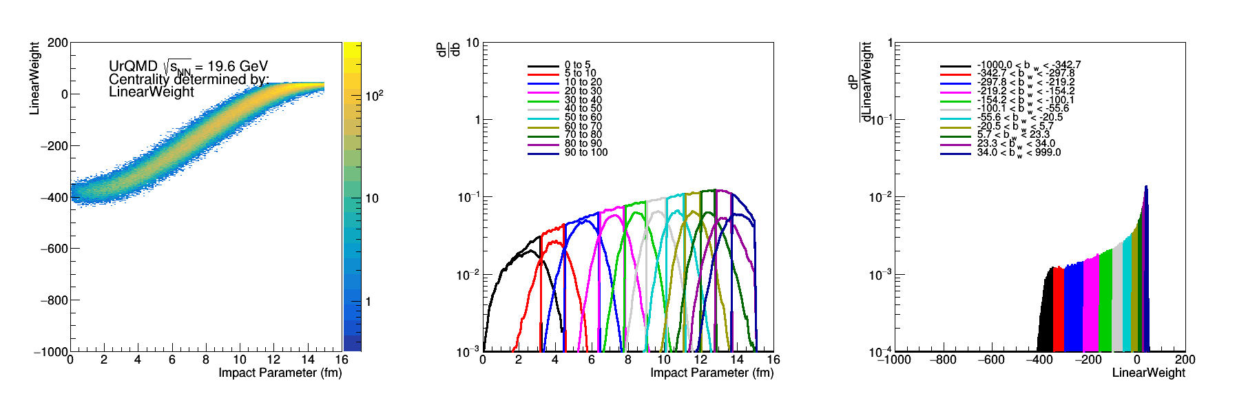
Figure 9: The left plot is the distribution of this covariance weighted b vs b, the middle is the distribution of the impact parameters for cuts in this b_{cw} and the right is the distribution of the cuts that I used.

This already looks nicer, so if we look at the sigma of the distributions again -

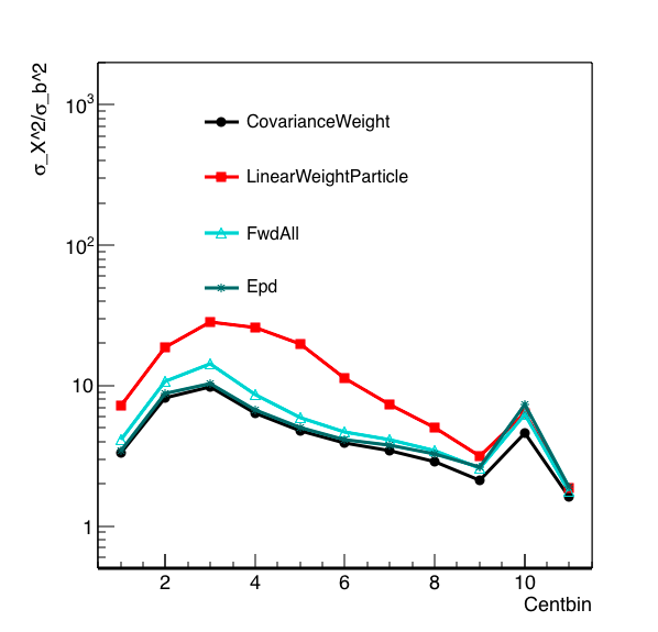
Figure 10: Sigma_x^2/sigma_b^2 vs centrality.  Most central events on the right, peripheral on the left.

The covariance distribution at least improves things to the point where the resolution is better than simple counting at the central end, and as good as simple counting for the peripheral bins.  There is a natural weighting by the number of hits in a given ring (weight x 0 = 0 for example), but this is naturally weighing each ring outside of the second ring nearly the same as the magnitude of the correlation factor is similar.

This could actually be an issue for the most peripheral events as the ring 1 distribution saturates due to the particle count, and thus loses resolution, but the other rings have very few counts so would not contribute.