Abstract:  Based on EEmc Gammas via conversion method, retool from previous attempt at extracting yields, we generate a new MC sample.

 

Event sample:

Notes:

1) The gamma maker cuts gamma candidates below a reconstructed pT < 3.0 GeV [default is 5 GeV].  It also requires an identified vertex.

2) Since we generated flat in pT, the efficiencies will not be reliable near threshold.  So we will need to make a cut > 8 GeV or so when we compare yields in data to pythia projections.

3) Four jobs (4, 28, 31, 39) hung unexpectedly.  We do not use these four files.

 

Our eventual goal is to compare yields extracted from the data for a fixed luminosity sample to projections from pythia.  (Ultimately to calculate a cross section, d2(sigma)/d(eta)d(pT) in one eta bin which encompasses 1 < eta < 2).

 

Let's start by looking at a subsample (about 1/2) of the events generated above.  We want to see how many events are identified by the gamma finder, and where any subsequent losses are.

 

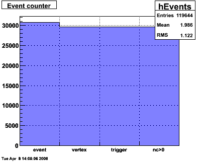
Figure 1.1 -- Number of events vs. event cuts.  Events correspond to a single, simulated collision.

 

 

Observations:

1. 30k events in this subsample.

2. <1% of these events fail to find a vertex.

3. The "trigger" column shows fraction of events which satisfies the selection on trigger ID.  There is no selection on trigger ID made.

4. Every event w/ a vertex also has one or more gamma candidates

 

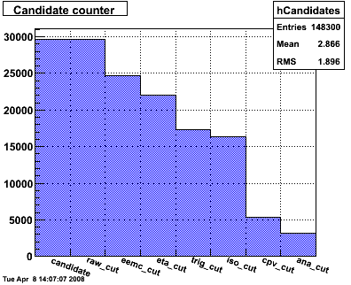
Next we look at the gamma candidates themselves.  Where do they get lost for given cuts in the analysis?  The cuts are applied in the following order:

 

1. Require that we have a candidate

2. raw_cut -- and it is not a null pointer

3. eemc_cut -- there is a gamma candidate reconstructed in the eemc w/ pT > 3 GeV

4. eta_cut -- the gamma candidate is w/in 1.0 < eta < 2.0  (real, not detector eta).

5. trig_cut -- the gamma candidate would satisfy the L2gamma component of the trigger.  http and bbc components not simulated.

6. iso_cut -- the gamma candidate satisfies the isolation cut  (90% of ET w/in R<0.3 in gamma candidate)

7. cpv_cut -- the gamma candidate satisfies the charged particle veto (Epre1 == 0 w/in R<0.3)

8. ana_cut -- the gamma candidate satisfies the analysis cut

 

Figure 1.2 -- Number of candidates versus cuts.

 

Observations:

1. Lots of ~10-20% losses add up.

2. For events which triggered, ~1/3 satisfy the CPV cut.  (5500/17k=32.3%).  This is ~consistent with Dave's analysis of photons identified from eta decays.

 

Next we plot efficiencies vs pT. 

Define: N_reco = The number of gammas which fallin w/in 1<eta<2,  satisfy the L2gamma component of the trigger (figure 2.1), and analysis cuts (figure 2.2).

Define: N_thrown = The number of gammas thrown w/in 1<eta<2

Then the efficiency is given by ε = N_reco / N_thrown.

 

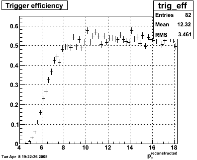
Figure 2.1 -- Something like a trigger efficiency vs reconstructed pT.  This is NOT a trigger efficincy (see below).  This is the number of events which hit the endcap, reconstruct with kinematics 1<eta<2, and satify the L2 compontent of the trigger DIVIDED BY the total number of events thrown w/ 1<eta<2.

Observations:

1. The "trigger" takes about 2.5 GeV to fully turn on.

2. Above 8 GeV, efficiency is essentiall flat.

 

"This is NOT a trigger efficiency".  The trigger efficiency would be calculated by counting the number of gammas which fired the trigger in a given pT bin, and dividing by the total number of gammas in that bin which hit the endcap.  What we have plotted above does that,...  but also folds in the acceptance, the resolution of the detector, the z-vertex smearing, a kinematic cut 1 < eta < 2, ... basically what we need to do to calculate a cross section.  So our real trigger efficiency is higher... hopefully tops out near 100% (but I need to measure this).

 

 

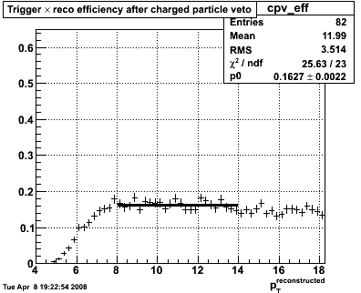
Figure 2.2 -- Efficiency for gamma candidates passing the (trigger) AND (isolation cut) AND (cpv cut).

Notes:

1. Efficiency is ~flat, and about 16% above pT > 8.0 GeV

2. Note that this means that ~30% of events which satisfied the trigger also pass the CPV cut.

3. This is crude.  The pT spectrum is steeply falling, but we threw flat.  (This was the only way to get the statistics in the time left).  There will be bin migration affects which are unaccounted for.  Expect efficiencies to go up a bit as events shift from right to left.  Yields will be overestimated.

 

 

 

When extracting yields from the data, it is important to treat two classes of events seperately.  Events with no energy in the postshower detector have a contribution from neutral hadron-initiated triggers which is small, but difficult at this point to quntify.  Events with nonzero energy in the postshower detector have a ~10% contamination from hadron-initiated triggers which we can correct for.

 

Based on EEmc Gammas via conversion method, systematics II we expect N(gamma) = 555 +/- 52 for pT > 8.0 GeV.

 

Based on EEmc Gammas via conversion method have a neglibible contribution for pT > 8.0 GeV.

 

Correct for a 16% efficiency for the CPV cut -- we estimate N(pt>8 GeV) = 3469 +/- 325.

 

Revised pythia estimates for 4.3 pb^-1 is 9000 events.

 

Conclusion: we are about a factor of 3 too low.

 

The  EEmc Gammas via conversion method, systematics II cited above had a few (~10%) jobs which failed.  Based on the full 4.3 pb^-1 sample we get

 

Extracted = 615.9 +/- 56.7

Eff. corrected = 3850 +/- 350

 

A factor of 2.3 lower than pythia.

 

Next, try binning everything above 8 GeV into a single bin to extract yield.

 

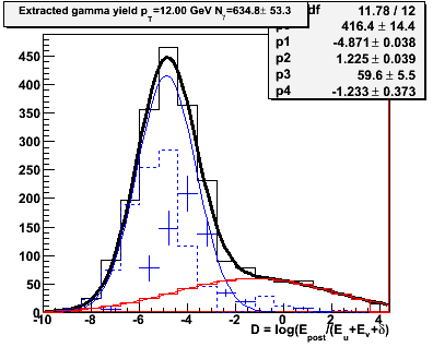
Figure 4.1 -- Extracted gamma yield vs "D", in a pT bin spanning 8.0 < pT < 16.0 GeV.

1. We get 634.8 +/ 53.3 events.  Compares well w/ extraction in multiple pT bins. 

 

1. Many runs in fill 7863 show up w/ partial file counts.

2. Several runs show up with no entries in histograms... most likely because the files don't exist at pdsf...

3. Few scattered "corrupt" runs, i.e. runs where (for one reason or another) root barfed.

4. Several runs w/ individual missing files.

5. There are several other runs which are in the list, but fast detector only?  e.g. 7145044.

 

catalgog query on jobs looked like--

<input URL = "catalog:pdsf.nersc.gov?runnumber=&run;,eemc=1,esmd=1,sanity=1,filename~st_phys,trgsetupname=ppProductionLong||ppProductionTrans,filetype=daq_reco_MuDst,storage!~HPSS" nFiles="all" />

 

yep... nothing in there to reject fast detectors only.

ok... so rewrite the catalog query and require TPC=1.
 

 

 

Therefore we need to (a) restrict analysis to only those runs which completed analysis of all files successfully, (b) recalculate luminsosity based on that run list.