Abstract: The
EEmc Gammas via conversion method for extracting single photons should, in principle, have easily quantified systematic uncertainties. One needs to know only two things -- the efficiency with which the signal and background pass the analyzing cut. In practice, since we have three sources of background, the systematic uncertainties become more complicated. We perform an extraction of the gamma yields vs pT, and determine the systematic uncertainties due to the measured efficiencies.
Contents:
0.0 Data Sample and Cuts
Event sample:
1. Data from ppLong2
2. All fills after L2gamma EEmc elevated to physics
4. Select trigger ID 137641
Cuts:
Before extraction:
1. Require candidate to be w/in the EEMC with pT > 5.0 GeV.
2. Isolation cut -- ET / ETR<0.3 > 0.9
3. Charged particle veto -- require sum of all preshower-1 tiles w/in R < 0.3 to be == 0
4. Analyzing cut -- sum preshower-2 tiles w/in R < 0.3 is greater than zero (i.e. at least one tile w/ ADC > 3 sigma + ped).
Post Extraction:
5. Extracted yields summed over -8 < D < -2.
1.0 The Efficiencies
We classify our backgrounds into two types: photonic backgrounds, which leave an experimental signature consistent with an electromagnetic shower, and hadronic backgrounds, which appear consistent with a hadronic shower. The efficiencies for these backgrounds are extracted directly from the data. The procedure is described
EEmc Gammas via conversion method, determine/cross check efficiencies. They were found to be:
εhadronic = 0.453 +/- 0.018
εphotonic = 0.940 +/- 0.007
The efficiency for single photons to pass the analyzing cut was determined using single-particle Monte Carlo. Its value was found to be
εgamma = 0.660 +/- 0.013.
The pT dependence of the hadronic background was shown to be negligible. The pT dependence of the photonic background has not been investiated. Neither has the pT dependence of the single photon efficiency.
2.0 The Method
The method is described.
Table 2.1 -- Definition of pT bins.
| Bin |
min pT [GeV] |
max pT [GeV] |
| 2,2 |
5.0 |
6.0 |
| 3,3 |
6.0 |
7.0 |
| 4,4 |
7.0 |
8.0 |
| 5,6 |
8.0 |
10.0 |
| 7,8 |
10.0 |
12.0 |
| 9,12 |
12.0 |
16.0 |
2.1 Estimate the fraction of hadronic background in the pT bin
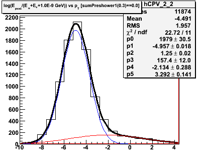
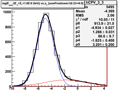
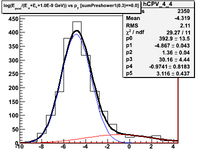
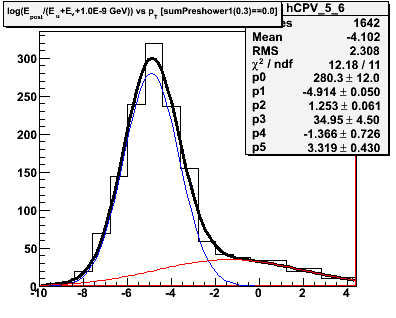
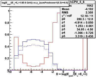
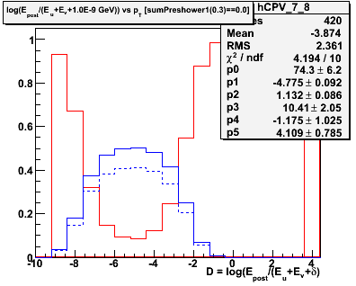
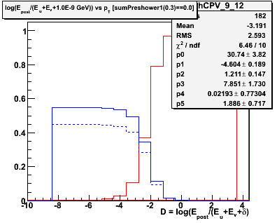
Since there are two known sources of background in the event sample, the efficiency for "background" events will change as the composition of that background changes. Our first task is to estimate how much of each type of background is present in any pT bin. The variable D = log(Epost/Esmd) tests whether the candidate looks "photon-like" vs "hadron-like". i.e. large energy in the SMD and relatively small postshower energy indicates an electromagnetic shower. Large postshower energy relative to the SMD energy indicates a hadronic shower.
Figure 2.1 -- Initial background estimate for gammas + photonic background (blue function) and hadronic background (red function). We plot the number of events vs
D = log(Epost/Esmd).
Observations:
1. Chi^2 is good in some pT bins, poorer in others.
2. The estimated hadronic component in the last pT exhibits a different behavior than in the other bins. We may need and/or want to parameterize the evolution of this function and fix some parameters.
3. We now have in hand an estimate of the percentage of hadronic background is in our spectrum. We do not yet know how to come up with an average efficiency for the combined background. This is the next step in the calculation.
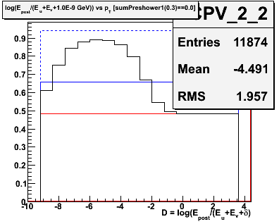
2.2 Intial estimate of single-gamma to photonic background
We have an estimate of the hadronic background component above. Our goal is to determine an estimate for the photonic background (i.e. pi0-->2 gamma, jets with multiple gammas which pass our cuts, etc...), so that we can average the two to determine the background efficiency. Since we don't know how to divide up the number of events beneath the blue lines in figure 2.1, we make a guess. We assign 60% of the fit yield to single gammas, the rest to the background process.
Figure 2.2 -- Initial decomposition of the spectrum. We plot the fraction of each of the three components in the spectrum. Solid blue for the single gammas. Dashed blue for the photonic background. Solid red for the hadronic background. The events in the gaussian have been split 60/40 between gammas and photonic background.
Observations:
1. The initial estimate for the composition of the background varies quite a bit. This probably reinforces the desire to reduce the number of free parameters in the fits in section 2.1.
2. Cutting events with D < -8.0 || D > -3.0 may be needed for other analyzes (i.e. the shower-shape analysis). It depends on whether the general behavior of the fits in section 2.1 is to be believed or not. Ultimately this will need to be addressed by the Monte Carlo.
3. With an estimate of the fraction of each type of event, we can now compute the average efficiency with which a background event passes the analyzing cut.
2.3 Efficiency for backgrounds to pass the analyzing cut
For each bin in the variable D, we now have an initial guess as to how many of each type of background which we have. We also know the
efficiencies for each type of background. In principle, all that remains is to do the following --
1. Calculate the efficiency, averaged over the background components, in each bin in D
εbackground = fphotonic × εphotonic + fhadronic × εhadronic
2. Knowing the background efficiency, determine how many events which satisfied the CPV cut pass the analyzing cut. This gives us ε, and we can apply
Ngamma = Ntotal × (ε - εbackground) / (εgamma - εbackground)
to extract out the yield of single photons.
However, as figure 2.3 is about to illustrate, there is a problem with this scheme --
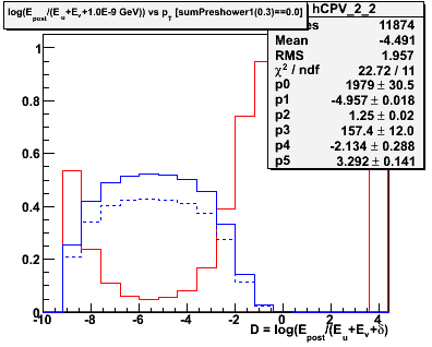
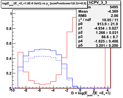
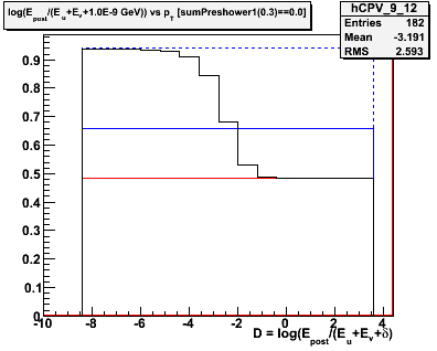
Figure 2.3 -- Average background efficiency vs D for the first (left) and last (right) pT bin. The solid black histogram denotes the background efficiency, averaged between the photonic background efficiency (dashed blue line) and hadronic background efficiency (solid red line). The single gamma efficiency is denoted by the solid red line.
Figure 2.3 illustrates a problem with the extraction method. The background efficiency becomes equal to the single photon efficiency as we move across in D. Why is this a problem? Because the equation which we use to extract the photon yield is
Ngamma = NCPV × (ε - εbackground) / (εgamma - εbackground)
which is not well behaved when the photon and background efficiencies are equal. At this point, there is no dicrimination power in the algorithm at all, and the answer is simply undefined.
Therefore we employ an alternate scheme. Instead of extracting the number of single-gammas vs D, we will extract the number of photonic background events. Then, using our estimate of the hadronic background yield from the fits in figure 2.1, we can estimate the single gamma yield. In other words --
Scheme for extracting single gamma yield in the presence of two backgrounds:
1. Compue the efficiency with which a single gamma or a hadronic background event will pass the analyzing cut
εγ+h = εgamma+hadronic = fgamma × εgamma + fhadronic × εhadronic.
2. In each bin of D in figure 2.1, compute
Nphotonic = NCPV × (ε - εγ+h) / (εphotonic - εγ+h).
3. Then compute
Ngamma = NCPV - Nphotonic - Nhadronic
where we take Nhadronic from the fit in figure 2.1.
4. The estimate of εγ+h may now be improved using the updated number of photons and photonic background events.
εγ+h = (Ngamma/NCPV) × εgamma + (Nhadronic/NCPV) × εhadronic.
5. With an improved estimate for the εγ+h efficiency, we can repeat the extraction in step 2 and get a better estimate of the yields. This procedure is then iterated to extract a final estimate of the gamma yields.
2.4 Extracted yields in each pT bin
Following the procedure outlined in section 2.3, we extract yields in each pT bin.
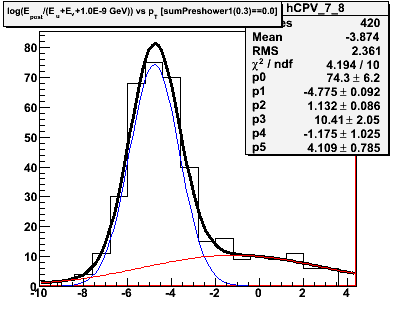
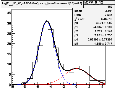
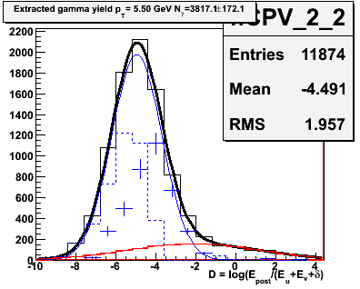
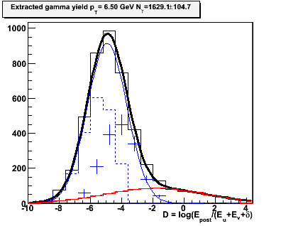
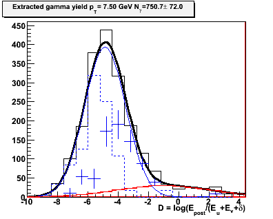
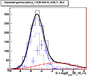
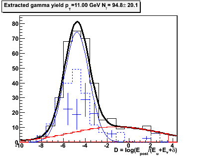
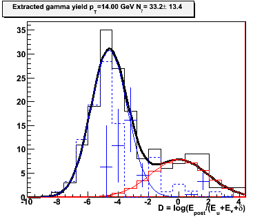
Figure 2.4 -- Yield extraction in each pT bin. The black histogram is the number of events which pass the CPV cut. Number which satisfy the analyzing cut are not shown. The blue data points are the extracted gamma yields. The dashed blue lines are the photonic background. The red line is the hadronic background estimated in the fits in figure 2.1... these are held fixed at every iteration.
Observations:
1. The gammas and photonic background seperate into two (unresolved) gaussian distributions. I suppose that this is reasonable to expect, since two photons from a pi0 decay should be better attenuated at the end of the calorimeter stack than a single gamma.
2. There are numerical "glitches" with this extraction scheme. For example, see the pT=11 GeV bin. At D>-2... I really don't believe that error bar. The uncertainty is being driven by the uncertainty in the fit, and the total number of events passing the CPV... but there are no pions in that bin. It looks like, once an iteration finds "no pions", all further iterations have "no pions". I don't think that's reasonable behavior, for an iteration to get "stuck".
Some QA:
1. The code converges on the same answer after 10 iterations as it does after 50. It is quicly convergent.
2. Verified that the extraction is insensitive to the inital composition. i.e. I varied the gamma/photonic background split in figure 2.2 from 95%/5% to 5%/95%, and checked that we reached the same result after 10 iterations.
3.0 Extracted pT Spectrum
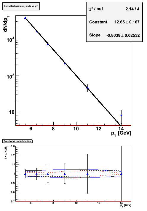
Figure 3.1 -- dN/dpT vs pT for single gammas. Top panel shows the pT spectrum. Bottom panel shows the fractional uncertainties (actually, 1 + the fractional uncertainties). The lines on the bottom panel show: (a) systematic uncertainty due to the +/- 0.7% uncertainty assumed for the photonic background conversion rate (dashed blue), (b) systematic uncertainty due to the +/- 1.8% uncertainty assumed for the hadronic background conversion rate (dashed red), and (c) the systematic uncertainty due to the +/-1.3% uncertainty assumed for the single gamma conversion rate.
Notes:
1. The statistical uncertainty on the extracted single gamma yield does not go like sqrt(N), because it has been background subtracted. Thus, the uncertainty on the 3800 events in the first pT bin is determined to be +/- 172, rather than +/- 62 as one might expect.
2. The stat. uncertainty on the data points depends on the number of photonic background events, and the number of hadronic background events, in each pT bin. Therefore, tighter SMD quality cuts will reduce the size of these uncertainties.
3. There are systematic uncertainties associated with determining the efficiencies for signal and background to pass the analyzing cut. The point of the second panel in the above figure is to determine how sensitive to these sysetamtic uncertaines the method is.
4. Systematic uncertainties are calculated by running the extraction code over the data with efficiencies increased / decreased by 1 sigma.
Observations:
1.The systematic uncertainties due to efficiency determination are almost constant w/ respect to pT.
2. At low pT, they are comparable with the statistical uncertainties. At high pT they are a negligible contribution to the overall uncertainty.
(In the 5-6 GeV bin, the systematic uncertainty added in quad. is 7%. Statistical is about 4%.)
3. It is not clear whether these uncertainties will cancel out, or to what level, when asymmetries are calculated. (My hunch is they will largely cancel).