Outline:

• Abstract
• Introduction
• The Problems
• Solution for Effect (1)
• Additional Observations for Effect (1)
• Solution for Effect (2)
• Solution for Effect (3)
• Putting the Pieces Together
• Using the Full Solution

 

ABSTRACT:

The context in which this came up is the question of whether Finding dead TPC regions (particularly FEEs or pads) within a TPC sector can bias the measurement of the GridLeak distortion. After some thought, I believe the answer is yes, and I have come up with some changes to the measurement we have been using which can reduce this bias, reducing systematic variance at the cost of increasing statistical variance. This is a welcome trade, as more data can be used to overcome statistical variance.

 

INTRODUCTION:

The method of GridLeak distortion measurement has traditionally been to take the difference of geometrically signed residuals of a pair of padrows on opposite sides of the inner/outer sector gap (i.e. padrows 12 and 14 with the old TPC electronics in Runs 1-8, and padrows 13 and 14 in Runs 9+). This generally works because of the following reasons:

1. The distortion moves hits in the inner sector in a direction opposite to hits in the outer sector. 
2. The distortion gives rise to residuals whose magnitudes are to first order proportional to the distortion itself (although there are second order effects, to be discussed soon),

Maps of the distortion making these points more clear can be seen GridLeak Distortion Maps.

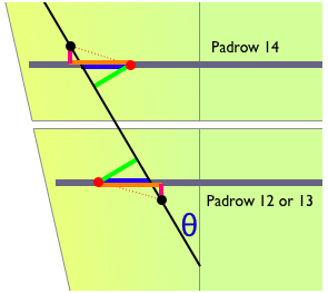
So despite the fact that the reconstructed track may not be in the same location as the original track, as long as the reconstructed track maintains an angle similar to the original track (a reasonable assumption given the nature and magnitude of the distortion compared to the length of the track), translations of the reconstructed track position have no impact on this difference. To demonstrate this point, the next pair of plots show a track reconstructed at two different locations: at its original location (left), and translated (right). The green bars represent the measured geometrically signed residuals to the reconstructed track (black line) from the reconstructed hits (red dots) on TPC padrows (gray bars).

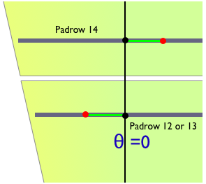
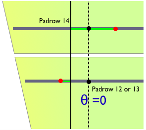
In these plots, θ is the angle between the track trajectory, and a line orthogonal to the padrows. The above plots show tracks with this trajectory angle θ=0.

 

THE PROBLEMS:

As noted, there are second order effects. These include:

1. As track trajectories become less orthogonal to the padrows (i.e. as |θ| increases), the magnitude of the residuals to the track decrease.
2. There is a small variation in the distortion magnitude as one moves from the middle of the sector towards the sector boundaries. The variation becomes particularly notable at the boundaries, which is why we do not use tracks and hits near the sector boundaries when measuring the distortion.
3. The distortion includes a component perpendicular to the padrows. This has no impact on tracks with θ=0, but contributes to the residuals along the padrow as |θ| increases.

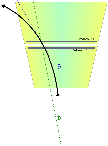
Effects 1 and 3 can be expressed by the following pair of plots, showing the distortion D (red dashed line) of the reconstructed hits (red dots) from the original hit positions (black dots), the measured residual (green), and the residual along the padrow (blue):

SOLUTION FOR EFFECT (1):

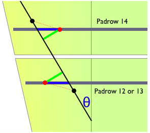
While we truly desire to measure the actual distortion, we can only measure hits at the padrows. So we do not really know where the black points lie when making the measurement. Both the usual residual R (shortest distance to the track) and the residual along the padrow R_row fail to perfectly identify the distortion magnitude, but it is apparent is that R_row has less sensitivity to the trajectory angle θ. Because θ is known (approximately, from tracking), determining R_row is a simple matter of dividing the usual residual by cos(θ).

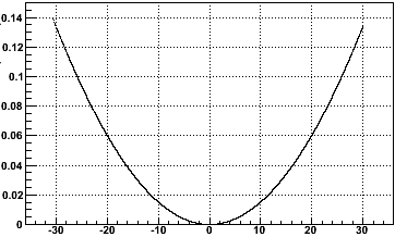
The usual residuals are underestimates of the residual along the padrow, and that underestimation grows with |θ|. Here is the fractional underestimate versus θ [degrees] (this is really just 1-cos(θ)):

Before going further, let us define φ as the angle between the center of the TPC sector and position where a padrow is crossed (measured about the center of the TPC).

Because only tracks which approach the primary vertex are used, the difference θ-φ is highly correlated with the p_T of the track, as shown here [degrees vs. GeV/c]:

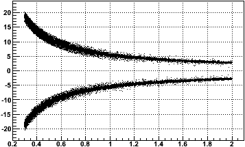
The two bands are the two charge signs, so the correlation is actually with q*p_T. This plot was generated with a real data sample of tracks used for measuring GridLeak, which explains the p_T cutoffs at 0.3 and 2.0 GeV/c.

For tracks at any given φ, the distribution of θ-φ will be reasonably constant in time for a dataset (as set by the q*p_T distribution). This dictates a correlation between θ and φ, implying that the underestimation in measuring the GridLeak with the usual residuals will also have a correlation with φ, or with position along the padrows.

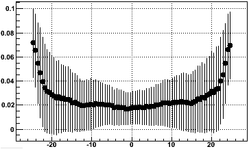
Using the same real data sample, this plot shows the correlation between the fractional underestimate and the distance from the center of padrow 14 at which the track crosses padrow 14 [cm] (where error bars represent spread, not error on the mean; cuts to avoid sector boundaries have already been applied in this sample):

Therefore, using residuals along the padrow will diminish the correlations between GridLeak measurements and position of tracks within the sectors. Because Finding dead TPC regions, the distribution of positions of tracks do vary from sector to sector. So this should also improve the uniformity of the GridLeak measurement from sector to sector.

 

ADDITIONAL OBSERVATIONS FOR EFFECT (1):

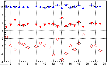
Using the same real data sample from Run 8 pp physics, which allows for weighting by real track distributions, we can see how the distributions for these relevant angles realistically compare from sector to sector. In the following plot, red circles are <φ>, red triangles are <abs(φ)>, and blue triangles are <abs(θ)> [degrees] vs. sector. Sectors 20 and 24 had dead regions preventing the measurement (Anode 20-5, RDO 20-2), as did sector 21 for some of the data (RDO 21-2). Sector 7 was excluded because a dead region (RDO 7-1) resulted in a poor measurement.

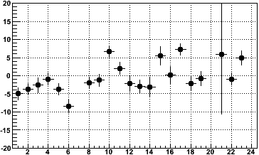
These translate into the following plot, which shows the fractional underestimate vs. sector. Blue and red points show the mean underestimates on padrows 14 and 12 respectively.

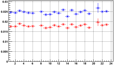
Systematic variation between sectors in the underestimate bias is clear, but only at the level of a few tenths of a percent. 

Integrating over all sectors, this is the underestimate on padrow 14 vs. Z [cm] using the same data sample:

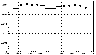
Again some systematic variation is clear at the level of a few tenths of a percent, and the symmetry between TPC halves gives confidence in it. As yet there is no hypothesis to explain this systematic. Nonetheless, it could be a factor in trying to observe linearity in the Z dependence of the distortion.

 

SOLUTION FOR EFFECT (2):

While effect (2) introduces a spread in the distortion measurements at a given Z, it would be something which we could ignore if all sectors had the same distribution of tracks across phi. But the previous section made it clear that this kind of uniformity does not exist in the Run 8 pp physics sample.

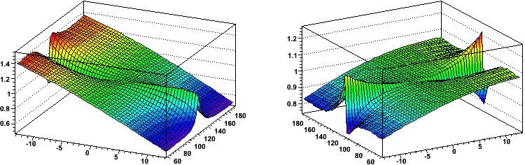
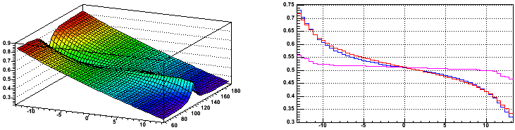
As the shape of the GridLeak distortion is believed to be GridLeak Distortion Maps and constant (though varying in magnitude with the amount of built up ionization charge density), we can scale all measurements to what we would expect at φ=0 (local X=0) to normalize out the distributions. The next two plots show the distortions in the local Y (perpendicular to padrow, left) and local X (along the padrow, right) directions vs. local Y [cm] and φ [degrees] normalized by the distortion at φ=0.

We are generally only interested in the distortions on padrows 14 and either 12 or 13. The following two plots are slices of the above plots close to these three padrows (blue: padrow 14; red: padrow 12; magenta: padrow 13), showing the normalized local Y and local X distortions versus φ [degrees]:

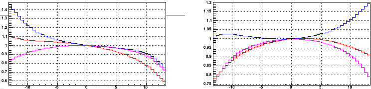
While it is still probably best to avoid getting close to the sector boundaries, using these scale factors should again improve the uniformity of the GridLeak distortion measurement from sector to sector. This correction factor (along the padrow) also appears to reach as much as 20% near one of the sector boundaries, and is asymmetric across the sector face. This turns out to be a much larger correction than effect (1). 

 

 

SOLUTION FOR EFFECT (3):

Effect (3) is a little bit more complicated. While the residual along the padrow R_row (blue line in the plot below) is less sensitive to θ than the usual residual R (green), what we really want is to measure the distortion D (red dashed line) or one of its components D_Y or D_X (magenta and orange lines respectively).

It should be re-noted here that the undistorted hits (black dots) may not really lie on the track as shown in the figure, but as long as the trajectory angle of the track is correct, translations do not matter. 

From the figure, we can see that the signed distortion component along the padrow D_X is equal to the signed residual along the padrow R_row plus tan(θ) times the distortion component orthogonal to the padrow D_Y. To keep signs correct, the above plot would have a positive signed residual on padrow 12 or 13, and thus a positive D_X, which implies a negative D_Y as drawn, so we actually want to subtract for that case; padrow 14 requires a plus to keep the proper signs. And in the previous section, we noted that we believe we know the shapes of the GridLeak distortion across the padrows, so we know the ratio D_Y ⁄ D_X even if we do not know their individual magnitudes.

S ≡ -1 {padrow ≤ 13}, +1 {padrow ≥ 14}
D_X = R_row + S D_Y tan(θ)
D_X = R_row + D_X S (D_Y ⁄ D_X) tan(θ)
D_X = R_row ⁄ (1 - S (D_Y ⁄ D_X) tan(θ))

where D_Y ⁄ D_X is a function of position and is as shown in the following plots, versus local Y [cm] and φ [degrees] (left), and versus φ [degrees] near the three padrows of interest (right; blue: padrow 14; red: padrow 12; magenta: padrow 13):

A flip in the magnetic field polarity will flip the sign of D_Y ⁄ D_X, so it does not require additional accounting in the formula. Again, this will advance the uniformity of the measurements, and may be a correction on the order of 10% as well.

We are almost done...

 

PUTTING THE PIECES TOGETHER:

Taking the results of the previous section another step further, the solution for effect (1) was to use R_row instead of the usual residual R. Since R_row = R ⁄ cos(θ), we can knock off both effects (1) and (3) by using as our measure:

D_X = (R ⁄ cos(θ)) ⁄ (1 - S (D_Y ⁄ D_X) tan(θ))
D_X = R ⁄ (cos(θ) - S (D_Y ⁄ D_X) sin(θ))

Let us define the following functions known from our distortion map shape, where X and Y are in local sector coordinates:

f(X,Y) ≡ D_Y(X,Y) ⁄ D_X(X,Y)
g(X,Y) ≡ D_X(0,Y) ⁄ D_X(X,Y)

Then we can use as our measure of the GridLeak distortion:

 D_X = g R ⁄ (cos(θ) - f S sin(θ)) 

where factors for effects (1), (2), and (3) are highlighted by color. Replacing the use of R with D_X should go a long ways towards reducing dependencies in the measurement of the GridLeak distortion on location within the sector where the measurement was made, and on trajectory angles of the tracks as they cross the padrows. The remaining places for potential errors are flaws in the distortion maps, and deviations in the angle of trajectory of the reconstructed track from the original track.

It is important to note that the solutions for effects (1) and (2) involved amplifying the measured residuals. The error on the measurement of the residuals involves the intrinsic errors of measuring hits and propagating tracks, and these errors are also amplified when making this scaling and will introduce statistical variance into the data where the scaling is greatest. The solution for effect (3) involves both amplification of some residuals and reduction of others. However, in terms of measurement errors its contributions remain additive, further increasing statistical variance. This should be understood as the cost for improved uniformity (reduced biases).

 

USING THE FULL SOLUTION:

Again using the Run 8 pp data sample, which has already been calibrated and corrected to some degree for SpaceCharge & GridLeak, we can look at the difference in GridLeak measurements made using D_X versus R from padrow 12 minus padrow 14 (looking at fractional under/overestimates does not work well for this comparison because the denominator in such a comparison may be very small). Here is the mean difference in measurements (measurement using D_X minus measurement using R) [microns] versus sector, where error bars are error on the mean, with typical RMS of ~150 microns for each sector:

M_diff = (D_X¹²-D_X¹⁴) - (R¹²-R¹⁴)

The fluctuation from sector to sector appears to be at the ±10 micron level on already-corrected data.

The same M_diff quantity [microns] integrated over all sectors versus Z [cm] is shown next:

Here we see a clear systematic again which undoubtedly impacts our interpretation of the slope of the Z dependence in determining GridLeak accurately. As before, a working hypothesis for this systematic is not yet known.

This plot has not been made for un-corrected data, but it is reasonable to expect that the differences grow with growing D_X and R. So it is poignant to see that even when data is believed to be reasonably well corrected, systematics at the level of tens of microns still exist when using the normal residuals R instead of our new estimator of the the distortion along the padrow D_X.

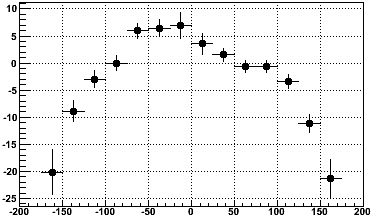
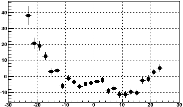
One final plot is M_diff [microns] versus distance from the axis up the middle of the sector [cm] at the supposed local Y of the distortion (121.8 cm) showing that the difference is clearly variable with position of the measurement across the face of the sectors, re-emphasizing the point that different dead regions in different sectors can lead to measurement biases:

 

_________________________________________________

FOOTNOTES:

1. The standard TPC definition of local X flips direction on opposite TPC halves, but was not flipped in this study.