- genevb's home page
- Posts
- 2025
- 2024
- 2023
- 2022
- September (1)
- 2021
- 2020
- 2019
- December (1)
- October (4)
- September (2)
- August (6)
- July (1)
- June (2)
- May (4)
- April (2)
- March (3)
- February (3)
- 2018
- 2017
- December (1)
- October (3)
- September (1)
- August (1)
- July (2)
- June (2)
- April (2)
- March (2)
- February (1)
- 2016
- November (2)
- September (1)
- August (2)
- July (1)
- June (2)
- May (2)
- April (1)
- March (5)
- February (2)
- January (1)
- 2015
- December (1)
- October (1)
- September (2)
- June (1)
- May (2)
- April (2)
- March (3)
- February (1)
- January (3)
- 2014
- December (2)
- October (2)
- September (2)
- August (3)
- July (2)
- June (2)
- May (2)
- April (9)
- March (2)
- February (2)
- January (1)
- 2013
- December (5)
- October (3)
- September (3)
- August (1)
- July (1)
- May (4)
- April (4)
- March (7)
- February (1)
- January (2)
- 2012
- December (2)
- November (6)
- October (2)
- September (3)
- August (7)
- July (2)
- June (1)
- May (3)
- April (1)
- March (2)
- February (1)
- 2011
- November (1)
- October (1)
- September (4)
- August (2)
- July (4)
- June (3)
- May (4)
- April (9)
- March (5)
- February (6)
- January (3)
- 2010
- December (3)
- November (6)
- October (3)
- September (1)
- August (5)
- July (1)
- June (4)
- May (1)
- April (2)
- March (2)
- February (4)
- January (2)
- 2009
- November (1)
- October (2)
- September (6)
- August (4)
- July (4)
- June (3)
- May (5)
- April (5)
- March (3)
- February (1)
- 2008
- 2005
- October (1)
- My blog
- Post new blog entry
- All blogs
DB efficiency in 24 hour stress tests
Following the 24 hour stress tests shown in the "Follow-up #4" section of Jerome's blog entry: Effect of stream data on database performance, a 2010 study, I looked a little further into the information I had regarding the DB efficiency in those productions (as measured by the ratio of cpu time spent on a job to the real, or "wall" clock time).
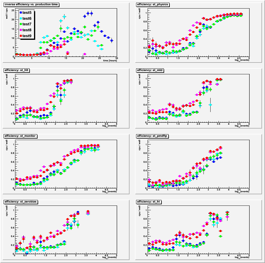
Here are the results, with the first plot showing similar information to what is seen on Jerome's page of wall time / cpu time, but merging all streams together and then overlaying the productions on top of each other. This is the wall time divided by the CPU time vs. production time (set so that 0 is approximately when the first job of the wave starts, and times are the start times of the jobs). I believe the labels "test5" through "test9", which come from Lidia's file and log locations, correspond to Jerome's tests 1 through 5 respectively. Tests 8 and 9 completed more quickly than the other tests, likely because of their improved efficiencies. Perhaps the only other notable thing in this plot is that test5 didn't begin to show inefficiency any sooner than tests 8 and 9. The plot looks pretty similar even using the finish time of the jobs instead of the start times.
The other seven plots are the DB efficiency vs. log10(events) for different streams. All streams, for all productions, show improved efficiency with larger numbers of events. While tests 8 and 9 show a clear improvement in efficiency for essentially any number of events (by factors of x3 or x4 at low numbers of events), what is apparent is that the number of events in the files plays as big a role as the actual stream or the DB setup. This is not news, but it re-emphasizes the point that small numbers of events in files is an important factor: regardless of the DB optimizations we have chosen, files with low numbers of events always make us inefficient.
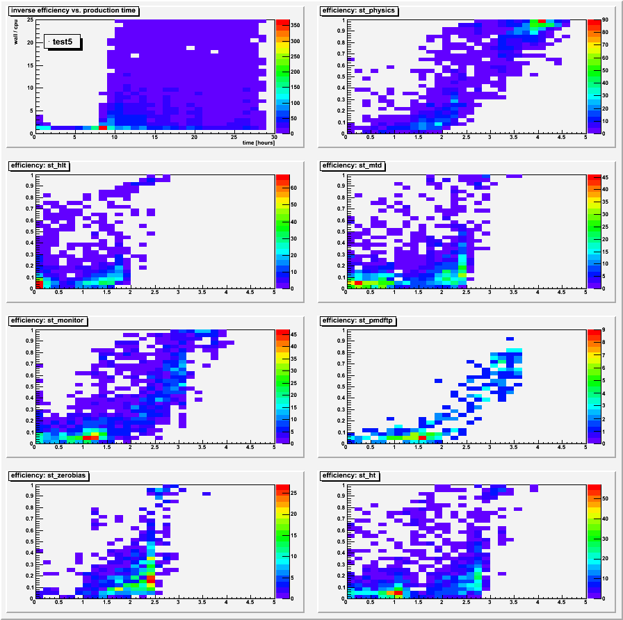
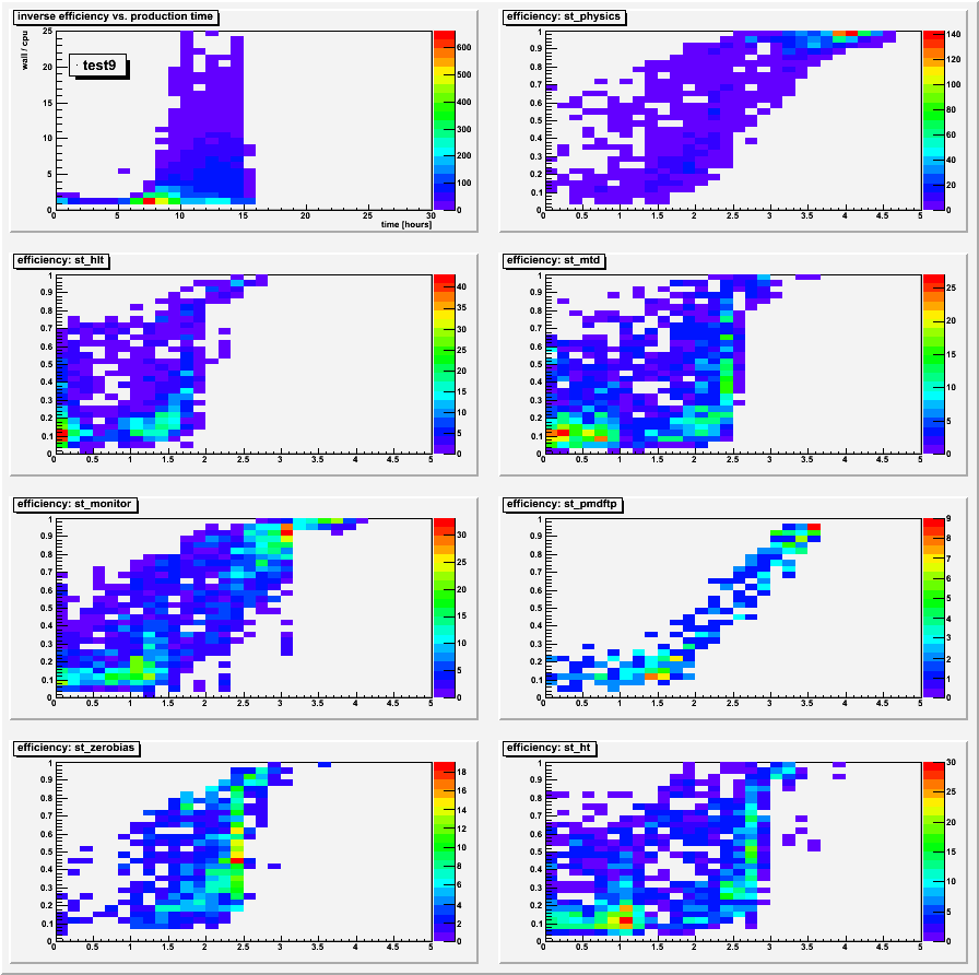
The second and third groups of plots below are zcol versions of the first group of plots, specifically for tests 5 and 9 respectively. They demonstrate that the profile plots reasonably depict the distributions; when stream data (not st_physics) files have lots of events, they are generally fine for DB efficiency as well. They tend to have many less events in their files than the st_physics data, thereby weighting themselves heavily in the inefficient region. Even within the st_physics data one can see two regions, and these correspond to the much less efficient st_physics_adc (low numbers of events) vs. non-adc files (lots of events).
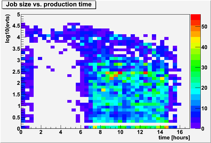
The very last plot shows that test9 began processing smaller size jobs (less events) about 6 to 7 hours into the production, which further explains the primary reason that this test started to show DB inefficiency for jobs starting about 7 hours into the production, getting increasingly worse as the small jobs continued.
-Gene
____________________________________________
Group 1: profile plots for all tests:
Group 2: zcol plots for test 5:
Group 3: zcol plots for test 9:
Job sizes (event counts):
Groups:
- genevb's blog
- Login or register to post comments