Effect of stream data on database performance, a 2010 study
Topics
- General introduction
- Results
- Follow-up #1
- Follow-up #2
- Follow-up #3
- Implementing first level idea (loading a portion of the DB for Run 10 a-la-Cloud)
- Follow-up #4 - MySQL partitioning test
- Action items
General introduction
Following a previous blog You do not have access to view this node, I asked Lidia to add to her own monitoring a separating by stream.
A quick run down of the problem: The issue was found as we processed the st_hlt files, believed to be done in a day but took a week+ to process. Inspecting the jobs, we then realized the ratio CPU/Real was terrifically disadvantageous. In addition, we also already observed that files with a low number of events would be inefficient for MSS access reasons.
The question are: can we do something to speed up stream processing? Can a combination of SSD, Memory and SAS can cure this issue?
- If YES, problem resolved and we will have more flexibilities ...
- If NOT, we would then have to
- All realize that taking streams does not equate to faster data production (on the contrary, switching to random time access of the database slow down dramatically)
- The only gain may still bring the benefits of faster user-end analysis.
- Solutions would include mixing streams and non-streams data (considering that _adc_ files may be as stream data as they are sampled sparsely in time) but preserving a time sequence while producing the files: for example, follow by RunNumber or sorting in time so we (a) do not get into a random access of tape into HPSS AND (b) we access the database from the streams and non-streams in an ordered time sequence. Remains to be known how the mixing would need to be for not losing too much efficiency (and can we re-order the events).
Results
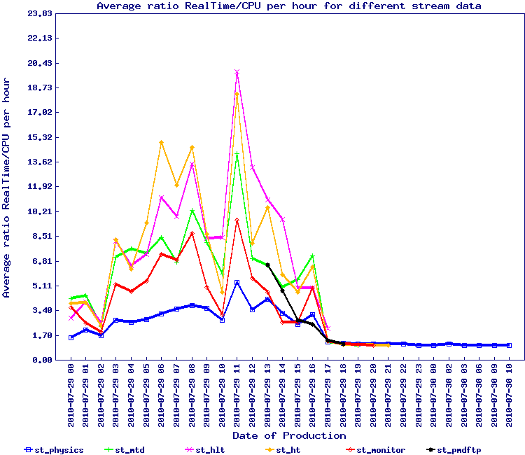
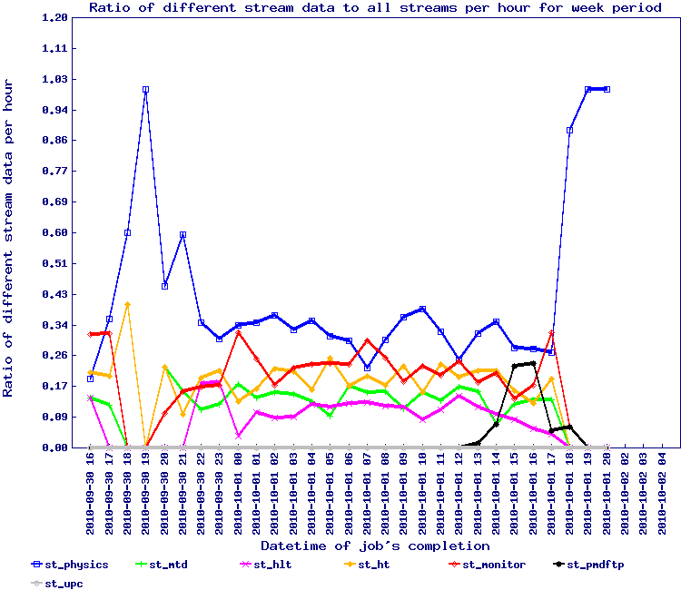
The plots below are the first view of this effort and represents files with at least 10 events in the file:
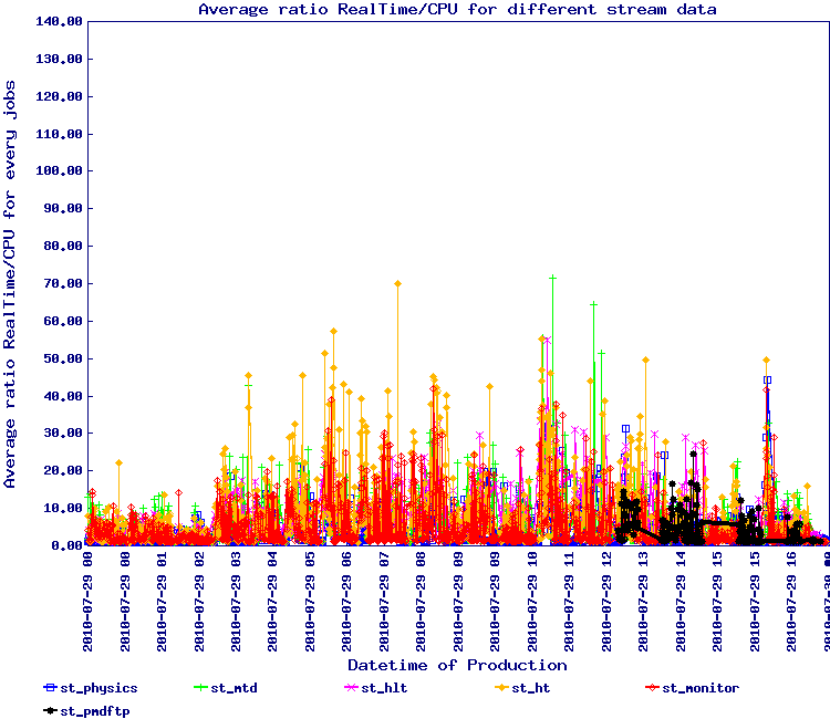
Observing the second plot, we see several outlier. Inspection and tracing identified a few by name:
- st_ht_adc_11123107_raw_1610001
- st_monitor_adc_11115089_raw_196000
- st_mtd_11115044_raw_1170001
Lidia also produced the list of files with the number of tracks and I digested this into the table below:
| Filename | <# tracks> | CPU / sec | RealTime / sec | # Events | CPU / Real |
| st_ht_11114055_raw_2150001 | 12 | 0.90 | 19.18 | 45 | 4.69% |
| st_mtd_11114057_raw_1190001 | 12 | 0.91 | 18.75 | 46 | 4.85% |
| st_mtd_11114057_raw_3190001 | 4 | 0.87 | 17.97 | 47 | 4.84% |
| st_mtd_11114057_raw_5180001 | 5 | 0.97 | 21.77 | 39 | 4.46% |
| st_physics_adc_11114084_raw_1500001 | 69 | 3.31 | 80.36 | 12 | 4.12% |
| st_ht_11114084_raw_4140001 | 9 | 0.77 | 21.34 | 52 | 3.61% |
| st_hlt_11114096_raw_3320001 | 60 | 2.05 | 59.08 | 23 | 3.47% |
| st_ht_11114109_raw_1140001 | 12 | 1.09 | 24.60 | 38 | 4.43% |
| st_pmdftp_adc_11114109_raw_1920001 | 90 | 3.71 | 91.27 | 12 | 4.06% |
| st_hlt_11114111_raw_3290001 | 80 | 3.52 | 86.77 | 12 | 4.06% |
| st_physics_adc_11114111_raw_3510001 | 65 | 1.52 | 36.10 | 41 | 4.21% |
| st_hlt_11114111_raw_5320001 | 60 | 2.43 | 64.42 | 19 | 3.77% |
| st_physics_adc_11114111_raw_5520001 | 53 | 1.85 | 57.81 | 29 | 3.20% |
| st_ht_adc_11114111_raw_5630001 | 2 | 3.37 | 71.18 | 13 | 4.73% |
| st_ht_adc_11114112_raw_2630001 | 5 | 2.86 | 69.58 | 13 | 4.11% |
| st_hlt_11114112_raw_3310001 | 109 | 1.98 | 53.14 | 37 | 3.73% |
| st_ht_adc_11115001_raw_2610001 | 24 | 3.17 | 91.71 | 14 | 3.46% |
| st_ht_adc_11115001_raw_5620001 | 3 | 3.36 | 93.82 | 11 | 3.58% |
| st_ht_11115005_raw_1150001 | 2 | 0.68 | 13.86 | 59 | 4.91% |
| st_mtd_11115005_raw_3170001 | 2 | 1.29 | 25.90 | 27 | 4.98% |
| st_ht_adc_11115006_raw_3640001 | 4 | 2.83 | 73.25 | 17 | 3.86% |
| st_ht_adc_11115007_raw_2610001 | 2 | 4.71 | 134.18 | 14 | 3.51% |
| st_ht_adc_11115007_raw_3610001 | 2 | 4.14 | 123.91 | 10 | 3.34% |
| st_monitor_adc_11115007_raw_3960001 | 199 | 4.59 | 125.50 | 10 | 3.66% |
| st_ht_adc_11115007_raw_4640001 | 3 | 3.10 | 107.28 | 12 | 2.89% |
| st_ht_adc_11115007_raw_5620001 | 3 | 2.87 | 74.51 | 13 | 3.85% |
| st_hlt_11115008_raw_4300001 | 94 | 2.05 | 52.20 | 33 | 3.93% |
| st_ht_adc_11115008_raw_4610001 | 13 | 2.04 | 48.15 | 20 | 4.24% |
| st_hlt_11115010_raw_1320001 | 278 | 4.71 | 102.55 | 13 | 4.59% |
| st_hlt_11115010_raw_3310001 | 138 | 4.64 | 144.44 | 10 | 3.21% |
| st_ht_adc_11115012_raw_4630001 | 4 | 2.69 | 133.15 | 14 | 2.02% |
| st_ht_adc_11115014_raw_3630001 | 9 | 3.06 | 62.14 | 12 | 4.92% |
| st_hlt_11115014_raw_4320001 | 65 | 3.07 | 93.26 | 14 | 3.29% |
| st_monitor_adc_11115015_raw_1950001 | 305 | 3.31 | 67.31 | 20 | 4.92% |
| st_monitor_adc_11115015_raw_2930001 | 141 | 3.00 | 86.23 | 19 | 3.48% |
| st_mtd_11115015_raw_3190001 | 7 | 0.38 | 7.74 | 252 | 4.91% |
| st_hlt_11115015_raw_4300001 | 114 | 2.33 | 54.25 | 25 | 4.29% |
| st_ht_adc_11115015_raw_4630001 | 1 | 2.40 | 49.23 | 16 | 4.88% |
| st_ht_adc_11115016_raw_3640001 | 12 | 2.45 | 108.13 | 20 | 2.27% |
| st_ht_adc_11115016_raw_5610001 | 2 | 2.74 | 63.47 | 14 | 4.32% |
| st_monitor_adc_11115016_raw_5960001 | 51 | 3.65 | 98.51 | 11 | 3.71% |
| st_ht_adc_11115017_raw_2620001 | 2 | 3.01 | 82.03 | 15 | 3.67% |
| st_ht_adc_11115017_raw_4610001 | 2 | 2.54 | 62.51 | 15 | 4.06% |
| st_monitor_adc_11115017_raw_4960001 | 233 | 4.18 | 94.02 | 12 | 4.45% |
| st_hlt_11115018_raw_1290001 | 76 | 1.67 | 55.54 | 38 | 3.01% |
| st_ht_adc_11115018_raw_1630001 | 2 | 2.58 | 87.67 | 15 | 2.94% |
| st_monitor_adc_11115018_raw_1940001 | 152 | 7.64 | 152.85 | 13 | 5.00% |
| st_ht_adc_11115018_raw_3630001 | 2 | 2.40 | 85.79 | 17 | 2.80% |
| st_monitor_adc_11115018_raw_3940001 | 224 | 4.58 | 167.71 | 10 | 2.73% |
| st_ht_adc_11115018_raw_4630001 | 6 | 2.94 | 138.05 | 16 | 2.13% |
| st_monitor_adc_11115018_raw_4940001 | 131 | 7.49 | 188.19 | 13 | 3.98% |
| st_ht_adc_11115018_raw_5630001 | 3 | 2.70 | 149.40 | 14 | 1.81% |
| st_ht_11115019_raw_1140001 | 14 | 0.61 | 26.82 | 94 | 2.27% |
| st_mtd_11115019_raw_1190001 | 3 | 1.32 | 84.94 | 27 | 1.55% |
| st_physics_adc_11115019_raw_1520001 | 79 | 3.44 | 75.57 | 26 | 4.55% |
| st_zerobias_adc_11115019_raw_1580001 | 1 | 1.47 | 39.63 | 32 | 3.71% |
| st_mtd_11115019_raw_2190001 | 9 | 1.16 | 31.99 | 33 | 3.63% |
| st_physics_adc_11115019_raw_2500001 | 74 | 3.30 | 72.95 | 24 | 4.52% |
| st_zerobias_adc_11115019_raw_2590001 | 5 | 1.16 | 28.25 | 50 | 4.11% |
| st_ht_11115019_raw_3130001 | 20 | 0.54 | 20.31 | 103 | 2.66% |
| st_mtd_11115019_raw_3200001 | 11 | 1.03 | 57.16 | 37 | 1.80% |
| st_hlt_11115019_raw_3290001 | 71 | 4.09 | 120.90 | 10 | 3.38% |
| st_zerobias_adc_11115019_raw_3590001 | 2 | 1.32 | 32.83 | 41 | 4.02% |
| st_ht_11115019_raw_4140001 | 5 | 0.50 | 17.13 | 96 | 2.92% |
| st_mtd_11115019_raw_4190001 | 54 | 0.93 | 20.53 | 52 | 4.53% |
| st_zerobias_adc_11115019_raw_4580001 | 2 | 1.18 | 29.20 | 48 | 4.04% |
| st_mtd_11115019_raw_5190001 | 16 | 0.99 | 28.78 | 40 | 3.44% |
| st_hlt_11115019_raw_5320001 | 76 | 3.49 | 83.45 | 12 | 4.18% |
| st_zerobias_adc_11115019_raw_5570001 | 3 | 1.33 | 31.44 | 39 | 4.23% |
| st_mtd_11115020_raw_1180001 | 6 | 0.38 | 9.97 | 152 | 3.81% |
| st_hlt_11115020_raw_1300001 | 33 | 2.82 | 58.40 | 14 | 4.83% |
| st_physics_adc_11115020_raw_1490001 | 54 | 1.69 | 54.06 | 34 | 3.13% |
| st_mtd_11115020_raw_2180001 | 3 | 0.37 | 7.85 | 159 | 4.71% |
| st_ht_adc_11115020_raw_2630001 | 2 | 5.42 | 145.18 | 15 | 3.73% |
| st_mtd_11115020_raw_3200001 | 6 | 0.35 | 8.09 | 180 | 4.33% |
| st_ht_adc_11115020_raw_3610001 | 19 | 3.32 | 113.84 | 13 | 2.92% |
| st_hlt_11115020_raw_4320001 | 45 | 3.08 | 168.77 | 13 | 1.82% |
| st_physics_adc_11115020_raw_4500001 | 71 | 3.43 | 72.19 | 24 | 4.75% |
| st_ht_adc_11115020_raw_4630001 | 9 | 3.22 | 68.82 | 12 | 4.68% |
| st_mtd_11115020_raw_5200001 | 5 | 0.36 | 10.01 | 179 | 3.60% |
| st_physics_adc_11115020_raw_5500001 | 70 | 2.00 | 62.84 | 30 | 3.18% |
| st_ht_adc_11115020_raw_5640001 | 6 | 3.54 | 123.59 | 10 | 2.86% |
| st_hlt_11115021_raw_1310001 | 86 | 1.83 | 42.33 | 45 | 4.32% |
| st_hlt_11115021_raw_2300001 | 70 | 1.58 | 45.01 | 41 | 3.51% |
| st_physics_adc_11115021_raw_2510001 | 69 | 1.15 | 25.44 | 106 | 4.52% |
| st_ht_adc_11115021_raw_2620001 | 3 | 3.08 | 77.19 | 15 | 3.99% |
| st_hlt_11115021_raw_3290001 | 69 | 1.60 | 42.54 | 42 | 3.76% |
| st_monitor_adc_11115021_raw_3930001 | 245 | 4.13 | 95.45 | 12 | 4.33% |
| st_ht_adc_11115021_raw_4630001 | 26 | 2.67 | 123.11 | 15 | 2.17% |
| st_hlt_11115022_raw_1290001 | 131 | 2.57 | 54.02 | 30 | 4.76% |
| st_ht_adc_11115022_raw_3620001 | 2 | 5.31 | 156.51 | 12 | 3.39% |
| st_ht_adc_11115022_raw_4620001 | 23 | 5.09 | 158.43 | 13 | 3.21% |
| st_mtd_adc_11115022_raw_4660001 | 2 | 3.12 | 222.57 | 12 | 1.40% |
| st_ht_adc_11115023_raw_4640001 | 4 | 2.19 | 81.13 | 19 | 2.70% |
| st_monitor_adc_11115023_raw_4950001 | 226 | 4.11 | 114.73 | 14 | 3.58% |
| st_ht_adc_11115023_raw_5620001 | 11 | 3.70 | 99.26 | 20 | 3.73% |
| st_monitor_adc_11115023_raw_5930001 | 217 | 3.74 | 141.93 | 16 | 2.64% |
| st_hlt_11115024_raw_1310001 | 114 | 3.05 | 98.71 | 17 | 3.09% |
| st_physics_adc_11115024_raw_1500001 | 131 | 2.16 | 45.36 | 36 | 4.76% |
| st_mtd_11115024_raw_5180001 | 6 | 0.57 | 18.62 | 81 | 3.06% |
| st_ht_11115025_raw_1130001 | 21 | 0.53 | 11.34 | 111 | 4.67% |
| st_ht_11115025_raw_2160001 | 8 | 0.49 | 10.93 | 99 | 4.48% |
| st_hlt_11115031_raw_2300001 | 153 | 4.70 | 95.95 | 10 | 4.90% |
| st_hlt_11115031_raw_4300001 | 62 | 4.13 | 100.81 | 10 | 4.10% |
| st_physics_adc_11115032_raw_2490001 | 75 | 2.22 | 56.62 | 26 | 3.92% |
| st_physics_adc_11115032_raw_3520001 | 90 | 2.23 | 46.24 | 29 | 4.82% |
| st_monitor_adc_11115033_raw_3950001 | 202 | 3.58 | 124.76 | 14 | 2.87% |
| st_hlt_11115039_raw_4310001 | 77 | 2.76 | 68.25 | 16 | 4.04% |
| st_hlt_11115039_raw_5310001 | 69 | 1.80 | 53.60 | 30 | 3.36% |
| st_monitor_adc_11115039_raw_5940001 | 199 | 3.58 | 92.08 | 14 | 3.89% |
| st_mtd_11115042_raw_2190001 | 3 | 0.88 | 26.09 | 43 | 3.37% |
| st_mtd_11115044_raw_1170001 | 2 | 2.41 | 123.89 | 15 | 1.95% |
| st_ht_adc_11115053_raw_1640001 | 1 | 2.25 | 78.96 | 18 | 2.85% |
| st_ht_adc_11115053_raw_5610001 | 2 | 4.32 | 166.67 | 10 | 2.59% |
| st_hlt_11115073_raw_4290001 | 70 | 1.50 | 43.36 | 58 | 3.46% |
| st_ht_adc_11115088_raw_3640001 | 2 | 3.66 | 75.06 | 10 | 4.88% |
| st_monitor_adc_11115089_raw_2930001 | 200 | 4.66 | 95.83 | 10 | 4.86% |
| st_monitor_adc_11116009_raw_4940001 | 262 | 3.70 | 89.49 | 21 | 4.13% |
| st_zerobias_adc_11123104_raw_1570001 | 31 | 2.17 | 51.22 | 20 | 4.24% |
More data is available from logs and the operation database. From that table, correlation should be extracted.
Follow-up #1
On 2010/08/04, we had a meeting and Gene presented additional plots (see You do not have access to view this node)and correlations (so no need to produce more from the above). The general conclusions were:
- We could narrow down the minimum number of events cut-off for optimal speed at 20 events per file
Status: done
- It was rather clear that the adc took more time than non-adc files (this was already showed based on average timing but even more strinking on 2D plots)
Status: checked - There are periods where everything is going well and there seem to be a time dependence (end of production had a bigger effect than at the beginning)
We discussed of not only the minimal number of events but what fraction of stream versus non-stream would be a beneficial threshold. The data would not show this but Lidia stated she could extract this information (Action item). Based on results, and in case the answer to the question above is NO, then this information would be useful.
I also brought several old topics and ideas we could try (now or in future):
- Trying to re-assess the use of memcache – no latency … but memcache may not be usable because it does not use timestamp but key=value
- Our timestamp need to be range, no problem because the key (in the key-value combo) could have the low and high time boundaries (+sdt timestamp) … and a tiered database storage used. By tiered database, one means that the workflow would work as follows:
- Query StDbMaker – is it cached there already? If the value is cached there, give it if not ...
- Build a string containing the low/high/sdt boundaries for the key query to memcache. Query memcache. Does it have the value? If yes, provide it. If not …
- Query MySQL, get value+boundaries+sdt back, build key and save into memcache
- This mechanism should be self-sustainable and dynamic providing that (a) we have as requirement that memcache entry lifetime could be set to large values and (b) that unpon a full cache, memcache could remove the oldest-entries-first and replace by new values. Then, there would be nearly no maintenance.
- As a side note, the key-value pair approach is similar to what we have as approach in database Web services SBIR with Tech-X
- Our timestamp need to be range, no problem because the key (in the key-value combo) could have the low and high time boundaries (+sdt timestamp) … and a tiered database storage used. By tiered database, one means that the workflow would work as follows:
- Second possibility and (already used) idea is to try the Cloud trick and have a MySQL server along with the job + a snaphsot (0.5 GB)
- This would imply we will have, as for Cloud, to manage the snapshot creation for every sdt we use + invent a “repository” mechanism if snapshot are the common mode of operation + modify our workflow to start (possibly stop) the DB with the proper snapshot (may not be immediate) and possibly start only one server per node (while there are many slots available)
- In a sense, memcache would be easier if self-maintainable (modulo the requirements already mentioned) as there would be no modifications of the production workflow
- We already know from Dmitry's performance study that a few thread access lead (not surprisingly) for faster response of the system ... we may be concerned of the rising number of slots per nodes.
- Third idea: if the assumption is that a database snapshot of 0.5 GB would fit in memory (file cache or otherwise, MySQL optimization), then we could
- Load a snapshot onto a few of our actual database servers
- Re-direct production jobs toward it
- Re-test and remake Lidia's plots above (we should see an immediate normalization of the time and efficiency as a function of streams)
- Some additional notes (relevant to the idea of one node = one MySQL service)
- The new node will have HT on and have twice the amount of memory …
- We have be careful of the Condor effect – not sure we can have on one node 16 jobs following each other in submission sequence and time. Even if we start with an initial time ordered distribution of jobs & slots, we will end up with some jobs finishing before others. Hence, some slots will be filled by jobs coming at a later point in time, ending with a complete random distribution of jobs & slots.
We discussed additional Action items:
- Implementing idea #3 which is immediate and not requiring any special infrastructure change (the loadBalancer may redirect to some servers, reshaped for the test of Run 10 data processing).
- Also pointed to Dmitry that while option #3 is immediate (a few reshape of the database, one trivial loadBalancer change and one snapshot to create at first for testing), option #1 and especially, thinking on how to implelement a Tiered database caching mechanism considering key=value would always remain useful.
If not for memcache, for any service relying on key=value (including Victor's trivial caching of the first snapshot only which could then be extended to multiple events).
Status: See this follow-up
Follow-up #2
On 2010/08/10, asked for feedback on action items.
- Lidia provided initial numbers for the cut at 20 events based on the 39 GeV data
- Lidia provided additional plots on the ratio of stream versus non-stream data
- Jerome followed up with Jeff on the adc issue - yes, adc are acting like stream data as initially thought (special conditions and selected once every N events, N being by the 100ds nowadays)
| stream | %tage of jobs with < 20 events / file | %tage events |
| st_upc | 65% | 4.6% |
| st_ht | 11% | 0.04% |
| st_hlt | 52% | 2.4% |
| st_mtd | 53% | 2.6% |
| st_monitor | 31% | 0.3% |
| st_physics | 10% | 0.006% |
| st_pmdftp | 17% | 0.04% |
Some conclusions:
- Rule (of Thumb): "The production team should consider regrouping production by runs and ordered time sequence and disregard guidance from PWG whenever the suggested production spans over multiple time sequence (this creates a random access to the database and exarcebate the issue)".
- Rule (of Thumb): "The production team will skip files with a #of events < 20 events/file as far as the total event loss will be < 4-5% (discretionary margin). Beyond this loss, the cut will be dropped to alternatively 15 then 10 events until the %tage of total event loss drops below the 4-5% indicated/allowed". This rule will be in addition of the already established "At 5% level of dying job for any given production series (by stream, by energy, by system, etc ...), the production team should not attempt to recover the dying jobs until production finishes. It will then be at their discretion on whether or not the loss should be recovered".
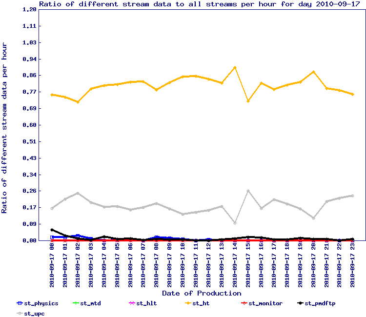
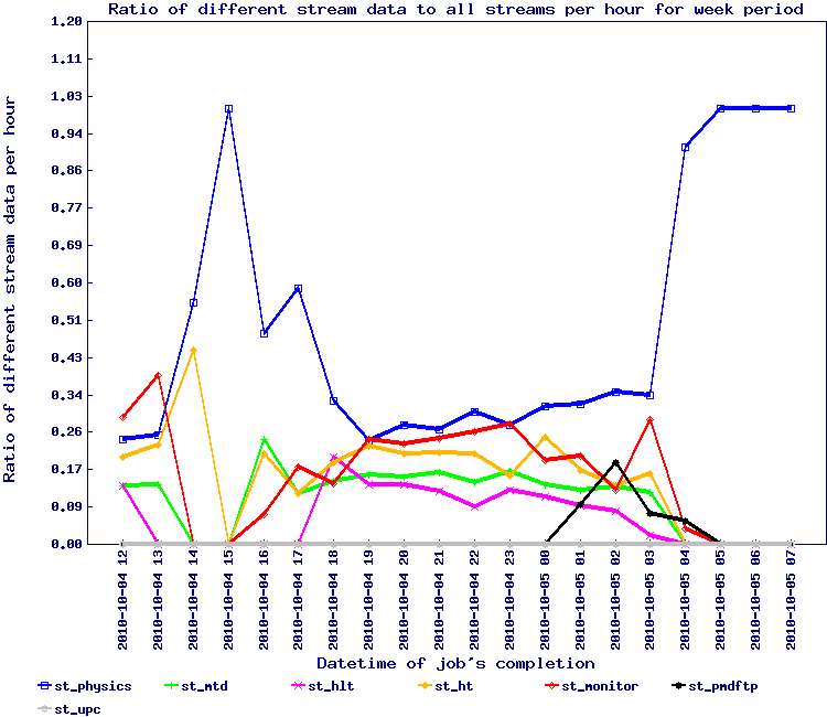
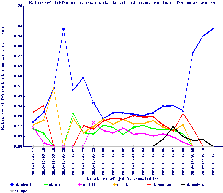
A small note on the first rule of thumb is the demonstration below that organizing by time sequence (grouping by run and time ordering jobs being submitted to the queue) has beneficial effects as noted.
In this test, the ratio / proportion of stream data is represented by the graph below
Follow-up #3
Dmitry presented an overview of the current status of the hyper-caching project (this is part of an SBIR with Tech-X Co. in large extent). A library is ready and could be implemented shortly modulo a few clean-up (redundant dependencies) and extension (retention and purge policies are not in place). Overall, clear that we are on track and there is no problem in understanding the key=value implementation.
One possible problem we re-discovered is that for the Web-service approach, passing SQL queries as the pseudo-protocol would not work because an efficient caching would need ot have information such as the validity range and the eventTime. Also, to be able to re-redirect to a separate service (in case of layered service and/or proxy chains), one needs to be able pass objects with embedded information otherwise, business logic of a a tiered-architecture software will need to spread at multiple places. Another obvious issue is that not using objects may force database-implementation specific logic (parsing, specific behavior logic) as well as experiment specific logic while object passing and a well defined communication protocol pushes all the db-specific logic at the lowest implementation layer (as it should) and experiment specific logic could be treated via a low level adapter (and a high level user front end BL). This is a bit technical and we decide to carry further this discussion in the context of the Tech-X SBIR.
No miss-understanding on the STAR side however - all inline with planning and general R&D idea.
Implementing the "third idea" (loading a portion of the DB for Run 10 a-la-Cloud)
This is similar to the cloud exercise but without the one MySQL server per node portion. The general notion is that a small enough database may be cached whole in memory, hence no delays in querries (random or ordered).
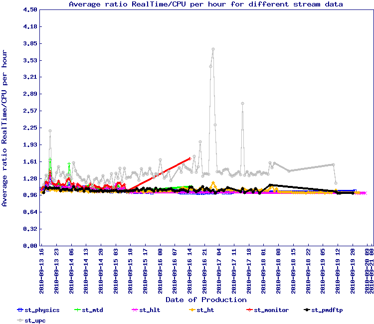
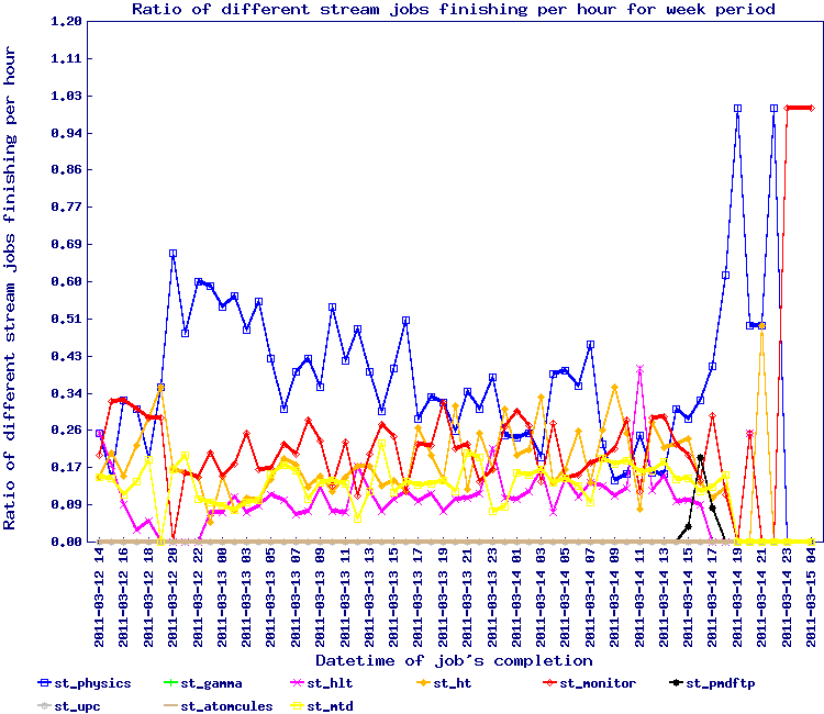
For the second wave of 7.7 GeV, we implemented the snapshot approach for Run 10 data and run from Monday the 16th to Wednesday the 18th of August. The results by stream is seen below.
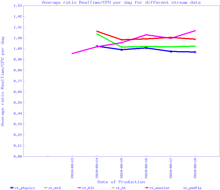
This test should need to be redone to be sure but overall, the efficiencies are back to 1.20 average i.e. an inverted ratio showing 85% efficiency or so. We can conclude this simple method seem to solve the issue.
To achieve this infrastructure, we can pursue a few options:
- Using Native MySQL partition table, fragment the calibration table into zones and by year (this solution is near immediate)
- Using a service realm separation (by port) and a redirect method to the proper data - this method is more aligned with a Web-service oriented architecture (and may be the longer term solution).
In all cases, the need to initialize the time line with startup values before a new Run and ending a run with stop values + inserting a simulation timeline before a new run is even more so important. Without it, separation by realm=year would not be possible. Which brings several Rule of Thumbs under perspective. They are all old principles but we violated them many times mainly due to "personal" (un-informed) preferences:
- "A real data run calibration timeline Y must be ended by stop values so a querry for data at timeline Y+1 would cause an immediate detection of problem"
- "Before each new run data period and timeline Y, calibration value entries must be initialized both for simulation adn real data: (a) the simulation entries must be entered at a time preceding a real data run by several months (b) we should not have real data (test data) values prior to the simulation timeline for year Y so we would not create miss-flavored entry effects (c) initialization values for real data must be entered in the database prior to a new real data run timeline but after the simulation timeline - such values may be copied from the detector state last known from the immediate previous run".
The above were already stressed when struggling with creating snapshots for the Cloud exercise at Clemson University (incidentally, the largest simulation wave we ever made in STAR, processing 12 Billion Pythia events).
Using native partition table from MySQL
MySQL 5.1 allows table horizontal partitioning based on a key belonging to a table. The statement ALTER TABLE ... PARTITION BY ... is available and is functional beginning with MySQL 5.1.6 so an on-the-fly reshape is possible. We would then partition by year so year 10 data queries would be confined to the partition reserved for year 10.
Horizontal partitioning allows a group of rows of a table to be written a different physical disk partitions (or at least, to a different file) allowing then to have underneath and managed by MySQL the same idea than the snapshot. No additional work on our side: if the entire partition in use would be cached as the snapshot, this would be an immediate improvement without further reshape of our infrastructure (and no special attention to building snapshots).
Note that to make this efficient, the rule of thumb of the previous sections still applies (if we have to fetch data from multiple partitions, we would kill the benefits).
Using service realm separation
A bit more tricky, this would best fit for Web-service approach whereas year (or even sub-system) would be available by service, where service is defined as server+port. This would require a redirection of some sort (hence the notion of WS and federated database starts kicking in naturally).
Follow-up #4 - MySQL partitioning test
50 jobs, partition table (nad baseline)
A test was defined at the end of August 2010, beginning of September to run ~ 50 jobs against db13, a standard STAR DB with a MySQL partitioned table with slicing on time periods (approximating the run periods).
The summary of this is test is pending. In general, some technical problems where encountered:
- Our job wrapper bfcca associated with Condor did not load the .cshrc and hence, we could not overwrite the definition of DB_SERVER_LOCAL_CONFIG . Condor does create a shell which loads neither .cshrc nor .login - This is under work.
- The first test attempted had all connections to the database server fail. It was unclear if this was related to a recent network reshape.
- The second tests started with 200 jobs and caused an overload (query rate to a single test DB) subsequently creating a large amount of reconnects. Reduced to 50 jobs, the behavior returned to a normal state.
The results were extracted for a single 50 jobs test but no reference was available.
On 2010/09/21, I have requested the following plan to be set in motion:
- Restart a test of the same 50 jobs toward the same db13 but with the standard MySQL (I would extend bfcca accordingly to allow redefining the DB load balancer configuration)
- If the results show improvements of the partition or no degradations, proceed with a partitioning of all DB services AND ...
- ... redo a test which would be comparable to our Results section (if not, we should re-run a baseline first, then go to partition tables and redo the test)
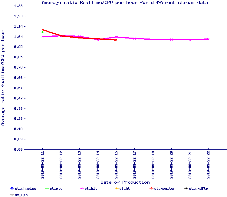
Result of the baseline at 50 jobs were available on 2010/09/22.
The load results from db13 were as below - this database was reverted to a normal setup since and put back into operational support for data production. Note the spike around week 35:
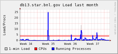
All jobs however ended in due time. The ratio results follow - on the left side, the result without partitioning and on the right, results with partitioning.
 |
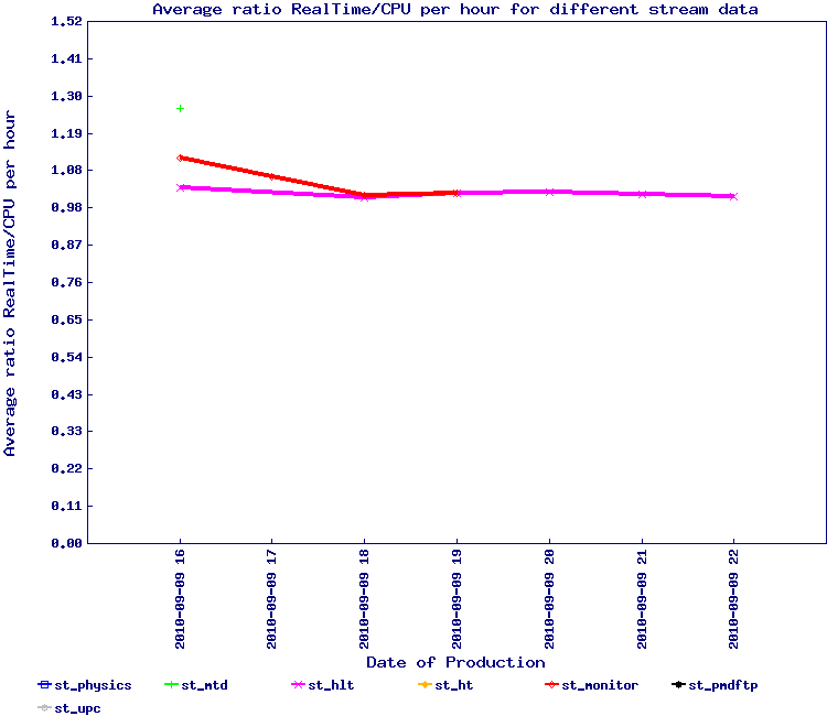 |
It would be tempting to conclude that the results are pretty similar to the "snapshot" method as described above but the number of streams were not as diverse. The baseline comparison (left hand side) is also pretty similar in performance.
24 hours stress test, wide stream representation
A test similar to the one above was designed to better quantify the effect of the database partitioning. The results are below with some observations:
| 1 | 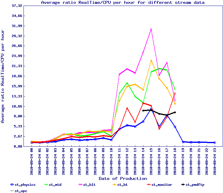 |
 |
| 2 | 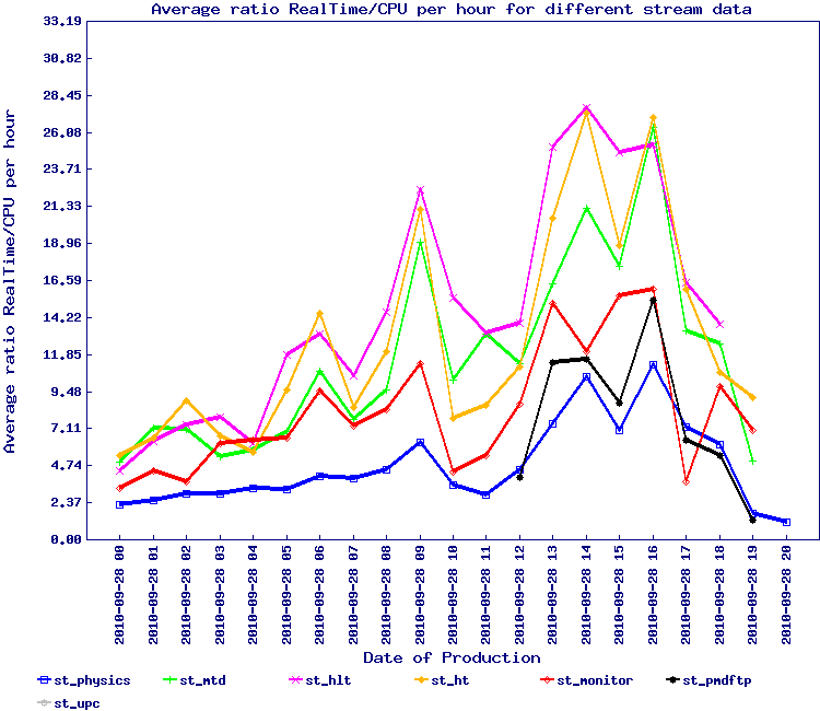 |
 |
| 3 | 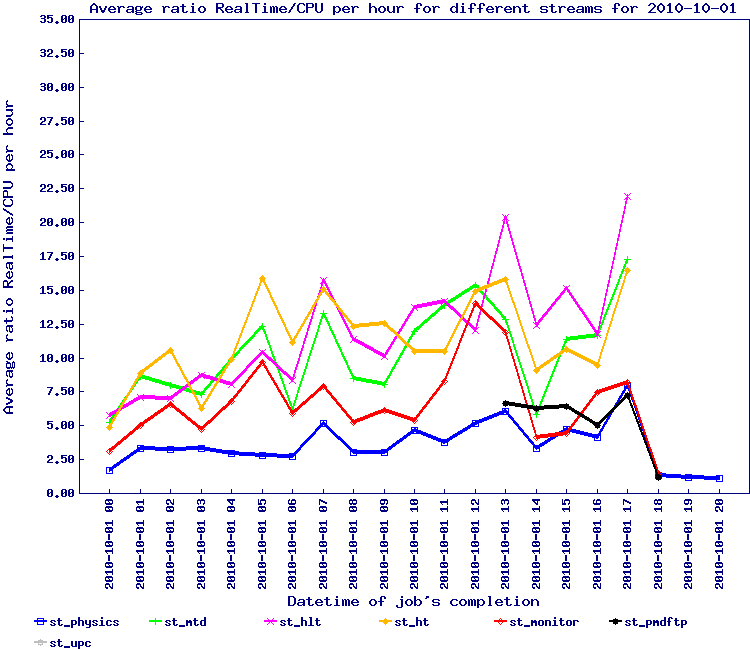 |
 |
| 4 | 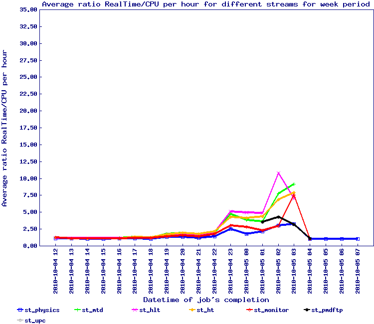 |
 |
| 5 | 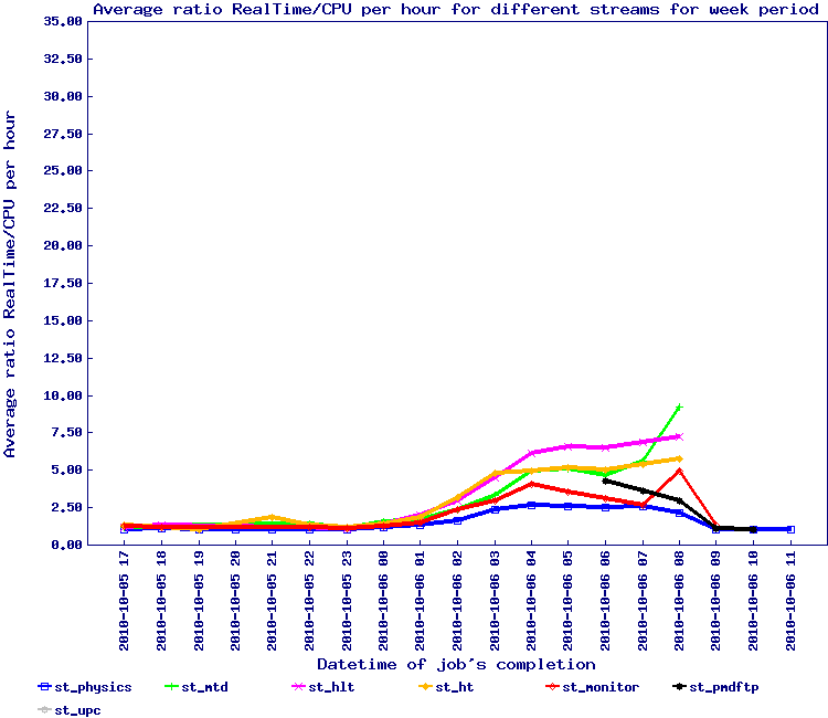 |
 |
| 6 | 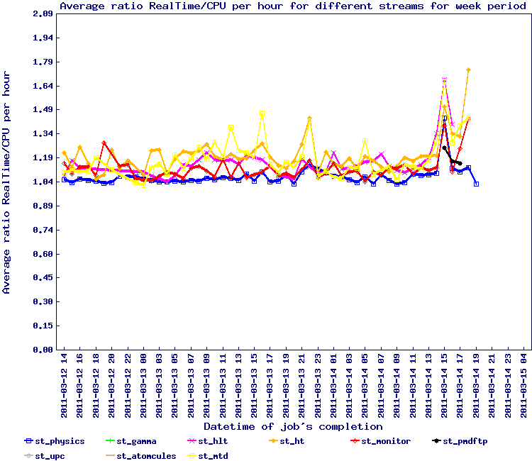 |
 |
- Base test - normal MySQL servers used with a job profile similar to our initial test and observations
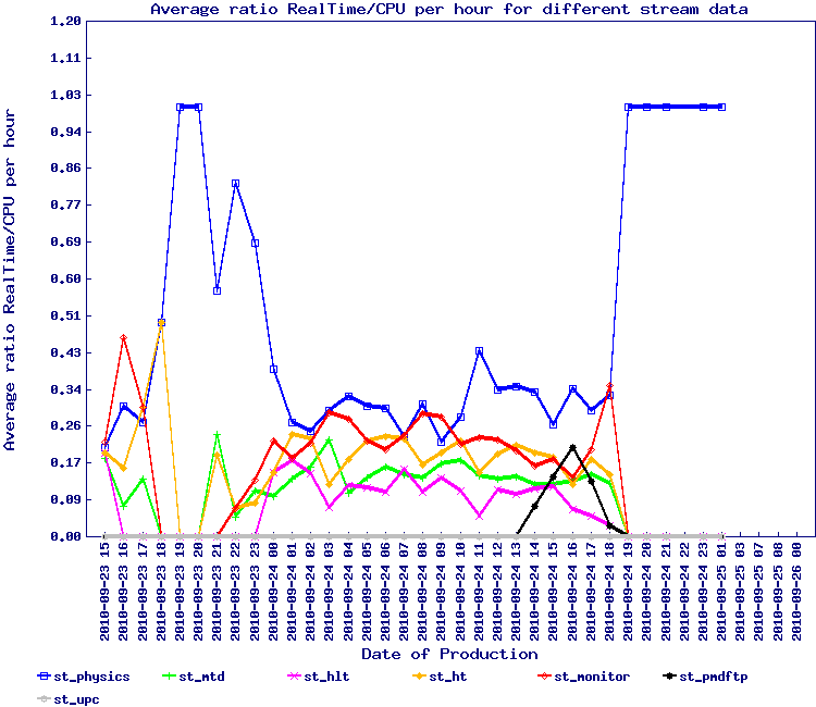
- Partition test 1 - MySQL servers used partition on date (isolation to year 10) - the jobs were sent to the queue in the same exact order than previously done. Several observations and notes:
- While the load overall seem to have decreased, this is very subjective and does not reach the level we expected (we expected a net relief of the ratio due to caching of the partition in memory)
- However, we had other jobs running in parallel (nightly tests), some of which used the database for the SSD data (year 5) hence forcing the DB to swap out the partition and replace. A third test with all nightly disabled was the decided (2010/09/28)
- Correlative: in future, and if a solution is found for this stream effect, all nightly should be isolated to their own service so they DO NOT interfere with normal data production.
- Partition test 2 - same as before but not nightly tests or other interferences.
Several observations:
- In this test however, a large amount of jobs died and the apparent drop in the ratio Real/CPU may only be due to the drop of load. In other words, job death at a rate was 26% would decrease the load on the server side.
- We attribute the job death rate to problems seen on the server side whenever partitioned tables are in use - resource consumption seem to grow and memory is exhausted, causing the server to abort the client request - the client aborts in the middle of a transfer and a segmentation violation occurs at our API level.
- Side note: Our API does not catch the server aborts (killed requests are not gracefully handled), a side lesson learn -> we need to check if this can be patched while fresh in our mind (we can easily reproduce this by killing client connections in action)
- Snapshot test 1 - in this case, the Cloud computing snapshot idea was put to use
Observations:
- First, we forgot to disable the nightly tests and it is possible that a remaining interference occurred - nightly tests starts at 3 AM and a definite ultimate peak is visible around that time (starting earlier)
- Additionally, database slaves are checked for integrity (sync check comparing to the master content) at 1 AM - at 1 AM, we see the ratio Real/CPU for the st_hlt stream starts to grow up
- However, and before that time, the test seems successful
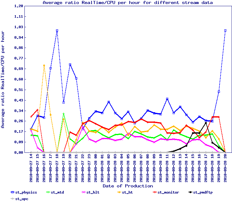
- Snapshot test 2 - same as before, no nightly, no integrity check
Observations:- Curve seems to flatten a bit but we still observe possible peaks of slow down at 7. This is however to contrast with the initial value of 35 (worst case scenario, we improved by a factor 5 comparing to the initial situation). It is also not clear what drives this slow down now as the increase started at ~ 02:00 AM (not corresponding to any special events) while there were no special change in the stream mix composition
- On the graphs saved in A load balancing study (stream test), there seem to be an event between 03:00-04:00 AM where the load on the server/service side drops comparing to previous and forward usage pattern (not sure I understand this over the full time period, even considering the job start differential). The load balancer otherwise did its work well.
- Running integrity checks on the DB have side effects in heavily loaded service scenario - we should think of disabling it whenever possible (if snapshots are used especially, no need for the integrity checkers)
- Test against new servers
- ...
Test from 2011/01/30
After the purchase of new nodes, a new test was made to understand how the increased memory and hardware would affect the access and load pattern. The following new graphs (based on the same jobs as above) were produced:
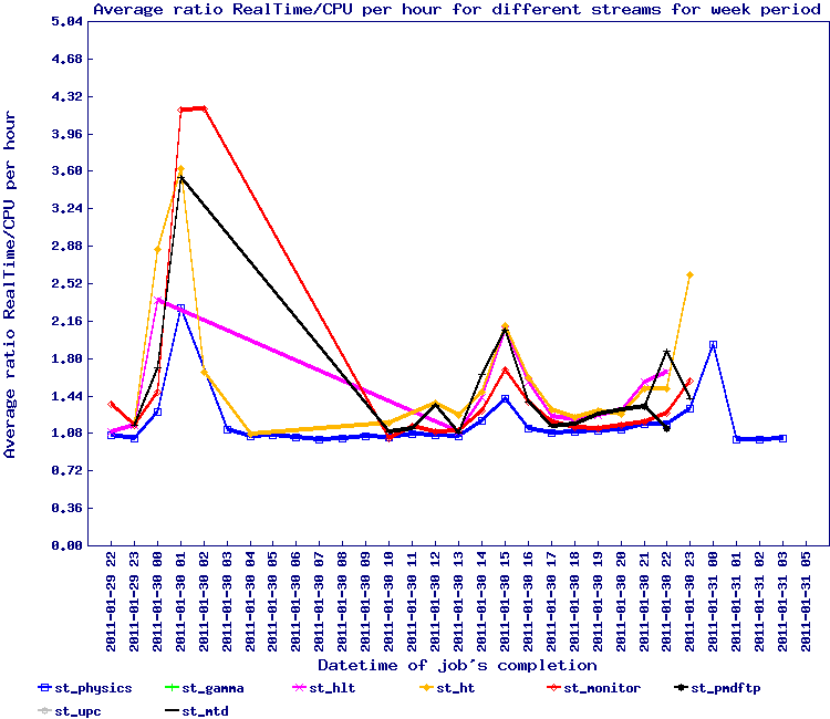 |
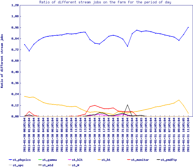 |
| CPU | Rate |
Action items
A summary of the rule of thumbs follows:
From the follow-up 2:
- Rule (of Thumb): "The production team should consider regrouping production by runs and ordered time sequence and disregard guidance from PWG whenever the suggested production spans over multiple time sequence (this creates a random access to the database and exacerbate the issue)".
- Rule (of Thumb): "The production team will skip files with a #of events < 20 events/file as far as the total event loss will be < 4-5% (discretionary margin). Beyond this loss, the cut will be dropped to alternatively 15 then 10 events until the %tage of total event loss drops below the 4-5% indicated/allowed". This rule will be in addition of the already established "At 5% level of dying job for any given production series (by stream, by energy, by system, etc ...), the production team should not attempt to recover the dying jobs until production finishes. It will then be at their discretion on whether or not the loss should be recovered".
From the follow-up 3:
- "A real data run calibration timeline Y must be ended by stop values so a querry for data at timeline Y+1 would cause an immediate detection of problem"
- "Before each new run data period and timeline Y, calibration value entries must be initialized both for simulation and real data: (a) the simulation entries must be entered at a time preceding a real data run by several months (b) we should not have real data (test data) values prior to the simulation timeline for year Y so we would not create miss-flavored entry effects (c) initialization values for real data must be entered in the database prior to a new real data run timeline but after the simulation timeline - such values may be copied from the detector state last known from the immediate previous run".
From 2011/02/03
- We found that restoring small files from HPSS actually breaks drives. The following rule then was set: Files with size < 150 MB should be removed from processing.
From the 24 hours tests:
- "In future, and if a solution is found for this stream effect, all nightly should be isolated to their own service so they DO NOT interfere with normal data production"
- Our API does not catch the server aborts (killed requests are not gracefully handled), a side lesson learn -> we need to check if this can be patched while fresh in our mind (we can easily reproduce this by killing client connections in action)
- Running integrity checks on the DB have side effects in heavily loaded service scenario - we should think of disabling it whenever possible (if snapshots are used especially, no need for the integrity checkers)
Consequent action items:
- jeromel's blog
- Login or register to post comments