- genevb's home page
- Posts
- 2025
- 2024
- 2023
- 2022
- September (1)
- 2021
- 2020
- 2019
- December (1)
- October (4)
- September (2)
- August (6)
- July (1)
- June (2)
- May (4)
- April (2)
- March (3)
- February (3)
- 2018
- 2017
- December (1)
- October (3)
- September (1)
- August (1)
- July (2)
- June (2)
- April (2)
- March (2)
- February (1)
- 2016
- November (2)
- September (1)
- August (2)
- July (1)
- June (2)
- May (2)
- April (1)
- March (5)
- February (2)
- January (1)
- 2015
- December (1)
- October (1)
- September (2)
- June (1)
- May (2)
- April (2)
- March (3)
- February (1)
- January (3)
- 2014
- December (2)
- October (2)
- September (2)
- August (3)
- July (2)
- June (2)
- May (2)
- April (9)
- March (2)
- February (2)
- January (1)
- 2013
- December (5)
- October (3)
- September (3)
- August (1)
- July (1)
- May (4)
- April (4)
- March (7)
- February (1)
- January (2)
- 2012
- December (2)
- November (6)
- October (2)
- September (3)
- August (7)
- July (2)
- June (1)
- May (3)
- April (1)
- March (2)
- February (1)
- 2011
- November (1)
- October (1)
- September (4)
- August (2)
- July (4)
- June (3)
- May (4)
- April (9)
- March (5)
- February (6)
- January (3)
- 2010
- December (3)
- November (6)
- October (3)
- September (1)
- August (5)
- July (1)
- June (4)
- May (1)
- April (2)
- March (2)
- February (4)
- January (2)
- 2009
- November (1)
- October (2)
- September (6)
- August (4)
- July (4)
- June (3)
- May (5)
- April (5)
- March (3)
- February (1)
- 2008
- 2005
- October (1)
- My blog
- Post new blog entry
- All blogs
Run 10 production times by dataset
Following on from A look at production times for AuAu 7 and 39 GeV, which focused on inefficiency of production jobs due to time spent accessing the DB, I tried to assess the computing resources needed for the Run 10 datasets based solely on CPU time per event (i.e. ignoring time spend waiting for DB response). This I have done by looking at items reported in a random sampling of production log files over the course of the past few months.
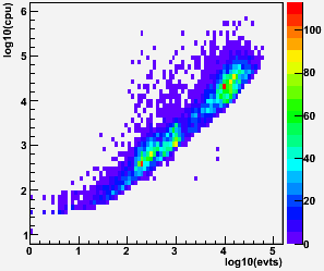
In the first set of plots, I show the raw distributions of CPU times for AuAu7 st_physics jobs versus the number of events in the jobs in the top left panel. The two large groupings of entries in the plot are from adc (lower event multiplicity) and non-adc (higher event multiplicity) files. As previously known, the files with just a few events are dominated by initialization. We decided after this to only produce files with at least 20 events (see Follow-up #1 on Effect of stream data on database performance, a 2010 study), and all other plots on this page will feature two things: (1) a cut on a minimum of 20 events in the job, and (2) a weighting of of data points by sqrt(# events).
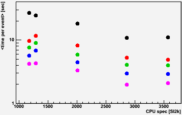
The lower left panel shows the mean CPU time per event versus the SI2k rating of the processors on which the jobs ran (obtained here) for st_physics jobs at each of the Run 10 collision energies (AuAu 200, 62, 39, 11, 7.7 GeV; lower energy events have lower multiplicity and so take less time to process). Statistical error bars are smaller than the markers. The plot demonstrates that CPU time per event can vary significantly (again, as expected) with the CPU spec rating.
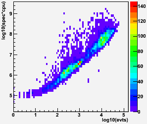
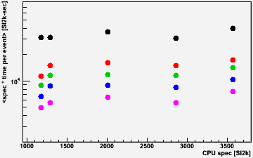
The plot in the lower right panel tries to normalize by multiplying the CPU time by the spec rating (this plot has the same vertical range of 40:1 as bottom left plot). This helps flatten the distributions significantly, with the exception of the nodes with 1169 SI2k rating which generally seem to outperform their spec despite also having the least amount of memory per core (1 GB; other nodes have 1 GB [1290 SI2k], 2 GB [1996 & 2862 SI2k], or 3 GB [3578 SI2k]). The upper right plot shows how the distribution tightens up using this metric.
| CPU time | CPU speed * time |
 |
 |
 |
 |
Now using the metric of spec * CPU time per event, it is important to recognize that there is still a notable spread in the performance metric for some of the data, as demonstrated by the following two plots. These are log10(spec * CPU time / event) [SI2k-sec] vs. stream ID (left and right axes respectively) for AuAu7 and AuAu39 (with the aforementioned cuts and weighting), where stream ID is in:
- st_physics
- st_ht
- st_gamma
- st_hlt
- st_mtd
- st_monitor
- st_pmdftp
- st_zerobias
- st_upc
- st_atomcules
Not all of these streams exist in all datasets (see tables below), and I have truncated these particular plots of stream ID 9 as I have no st_atomcules logs. Also, I have staggered adc files by offsetting them slightly (by 0.2) from these stream IDs.
| AuAu7 | 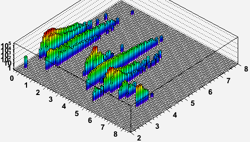 |
| AuAu39 | 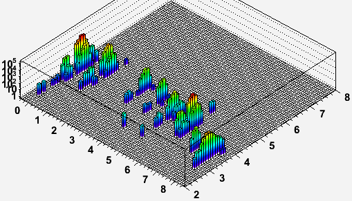 |
In the studied data, some of the AuAu7 streams have a very broad distribution extending up to approximately 10M SI2k-sec per event. Such jobs took several days (0.5M seconds!) to run and are almost certainly due to the observed Limiting production of events with large hit counts which cause a huge amount of time to be spent in the track finder. These long-running production jobs are not seen in the AuAu39 data. Unfortunately, there was no simple cut in this analysis to exclude such high multiplicity events or the jobs which processed them (though jobs which took even longer were killed in the production), and this will bias my results for the 7.7 GeV data.
Nevertheless, even the AuAu39 data show that some spread in resource needs per event exists between different jobs. The RMS of the metric is at about 20% of the measured means for AuAu39.
Anyhow, taking the mean of these weighted distributions yields the following numbers per event per stream, shown as a plot (statistical errors on the means shown, colors as before: AuAu 200, 62, 39, 11, 7.7 GeV) and a table. I only obtained log files for some of the streams, but the st_ht, st_hlt, and st_mtd streams show a clear bias towards more time per event than st_physics. Generally, the adc files also take a little longer thant the non-adc files.
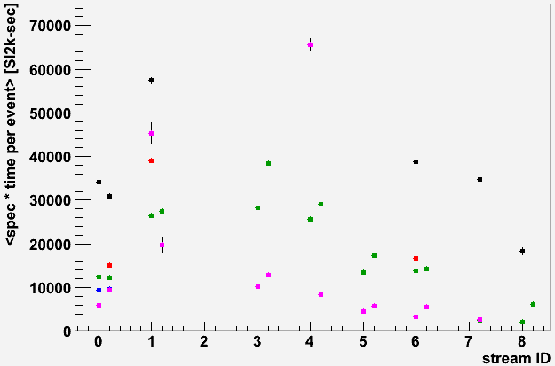
<spec * time / event> [SI2k-sec]:
| ID | stream | 200 | 62 | 39 | 11 | 7.7 |
|---|---|---|---|---|---|---|
| 0 | st_physics _adc |
|||||
| 1 | st_ht _adc |
|||||
| 2 | st_gamma _adc |
|||||
| 3 | st_hlt _adc |
|||||
| 4 | st_mtd _adc |
|||||
| 5 | st_monitor _adc |
|||||
| 6 | st_pmdftp _adc |
|||||
| 7 | st_zerobias _adc |
|||||
| 8 | st_upc _adc |
|||||
| 9 | st_atomcules _adc |
Event counts [M] as reported by the file catalog for AuAuX_production, where X is the collision energy:
| ID | stream | 200 | 62 | 39 | 11 | 7.7 |
|---|---|---|---|---|---|---|
| 0 | st_physics _adc |
690 14 |
191 4 |
253 5 |
1 |
2 |
| 1 | st_ht _adc |
59 1 |
0.7 |
0.3 |
||
| 2 | st_gamma _adc |
5 0.1 |
||||
| 3 | st_hlt _adc |
16 0.3 |
4 0.1 |
0.3 |
8 0.2 |
|
| 4 | st_mtd _adc |
15 0.3 |
3 0.1 |
1 0.0 |
0.4 0.1 |
0.9 0.0 |
| 5 | st_monitor _adc |
25 0.2 |
0.2 |
3 0.1 |
||
| 6 | st_pmdftp _adc |
0.1 |
4 0.1 |
23 0.5 |
||
| 7 | st_zerobias _adc |
0.0 2 |
0.0 0.6 |
0.0 |
0.4 |
0.0 1 |
| 8 | st_upc _adc |
38 0.8 |
3 0.1 |
0.4 |
||
| 9 | st_atomcules _adc |
17 0.3 |
1 0.0 |
|||
| Totals | 865 | 272 | 309 | 68 | 128 | |
Because I have many missing numbers, it's difficult to be accurate. But using some estimates from the above two tables, I arrive at the following approximate total CPU needs [SI2k-sec]:
200: 865M * 40k = 34.6G SI2k-sec
62: 272M * 18k = 4.9G SI2k-sec
39: 309M * 14k = 4.3G SI2k-sec
11: 68M * 9.4k = 0.6G SI2k-sec
7.7: 128M * 7k = 0.9G SI2k-sec
On a farm with approximately 3M SI2k available (essentially the current state, with only half of the rcas6xxx nodes plus all rcrs6xxx nodes available to production), and perhaps an 80% efficiency of completing jobs (e.g. service outages, failed jobs), these translate into the following time estimates for production:
200: 167 days
62: 24 days
39: 21 days
11: 3 days
7.7: 4 days
The pending arrival of new nodes to the farm should essentially double the available SI2k for production. At 6M SI2k, the 200 GeV production should be completed within 3 months of its start.
On a related note, $100k can procure a little over 0.4M SI2k. This would represent a less than 7% additional capacity for production (and less than 5% of the full RCF linux farm capacity) beyond the pending node arrival. That capacity could reduce the overall production time of AuAu200+39 by about 1 week.
-Gene
Groups:
- genevb's blog
- Login or register to post comments