The Event Plane Detector sees the Event Plane (and other quantities)
Updated on Sun, 2018-04-08 15:34. Originally created by lisa on 2018-04-08 12:58.
I have written code to analyze the muDsts and-- more importantly-- the picoDsts being produced by the Fast Offline jobs on the 2018 data. I will share this code with the "unblind" EPD analyzers, but wanted to make sure that it is working. Below I show some first plots.
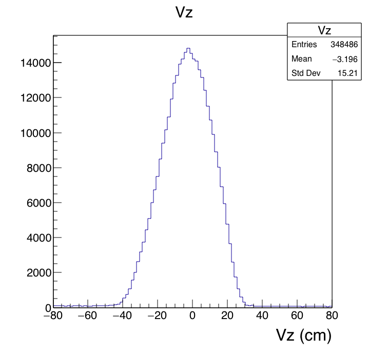
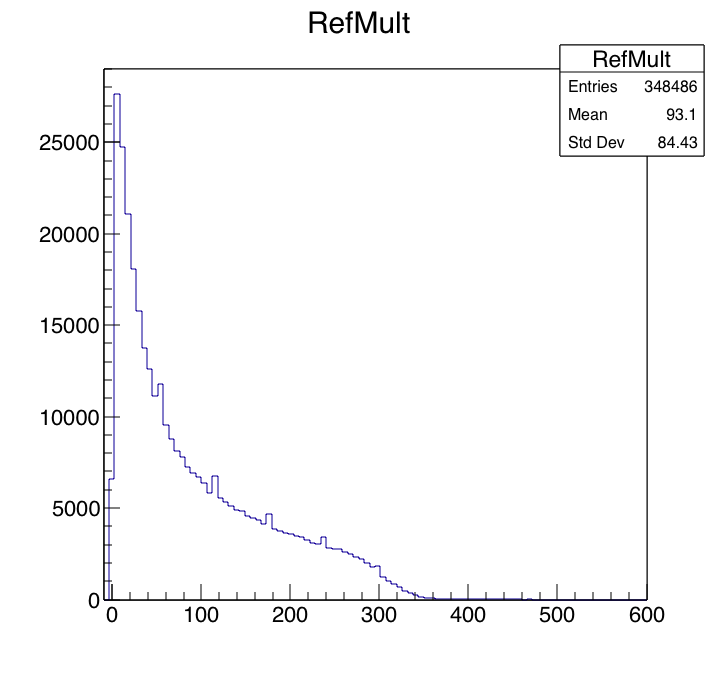
This comes from about 350 picoDst files, each holding about 1000 isobar collisions. Processing these 350K events takes about 2 wall-clock minutes on my mac. PicoDsts are definitely the way to go :-) Some global quantities first. (I suspect the small "spikes" in the RefMult plot are aliasing effects; I didn't look into it.)
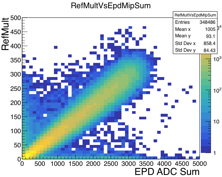
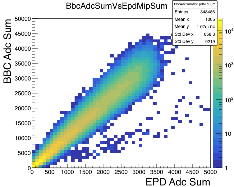
Next, just a quick look at the ADCsum in the EPD versus other measures of centrality like RefMult (in the TPC) and ADCsum in the BBC. (I'll update this with finer bins if I get time.)
Next, with the Event Plane Detector, we want to look at.... the Event Plane!
Keep in mind that "the" Event Plane is not unambiguously defined. Though I have worked with this data only for a short time, it is abundantly clear to me that there will be LOTS of opportunity for innovation, tuning, and algorithm development to optimize our resolution. This will be exciting.
For the moment, I stay with the simplest Q-vector analysis.
.png)
Usually the sum in these equations is over N particles. However, we have 744 tiles (many having zero signal in any given event). I loop over these tiles (called StPicoEpdHits in the STAR framework).
The angle \phi_i is given by the center of the tile. (Aside: why does this drupal editor even have a "special character" menu, if it doesn't have Greek letters??)
For the weight, wi, I use
.png)
This approach is driven by the understanding that large fluctuations in energy loss due to the Landau tail can actually degrade the quality of a global quantity. Hence, the requirement that the weight not be greater than some value Max does not throw away valuable information, but rather throws away distorting fluctuations. Or, anyway, it can. The data can tell us.
I did a little messing around, but not much. I just wanted to see that it works, and then we "unblinded folks" will play with the data some more. To avoid the tiles where the fixed-target holder produces an anisotropy (this could be corrected for, but I just cut it out to be quick) I use tiles with pseudorapidity<4. The pseudorapidity \eta_i is given by a straight line that connects the primary vertex to the center of the tile. (As I've mentioned several times, a tile is not associated with some given \eta or \eta range. One must specify the primary vertex and the tile.)
The 2nd-order event plane was reconstructed separately on the East and West wheels, and the full event plane resolution may be evaluated through their correlation:
.png)
(Yes, Dr. Isaac Upsal admonished me that the prefactor of sqrt(2) is only an approximation and that I should find the root of some function a la Voloshin & Poskanzer. I'm being lazy.)
First, the correlation between East and West. Okay, it's not beautiful enough to hold a parade over, but it's the first look and to me it's beautiful. We will be able to improve greatly, I am sure.
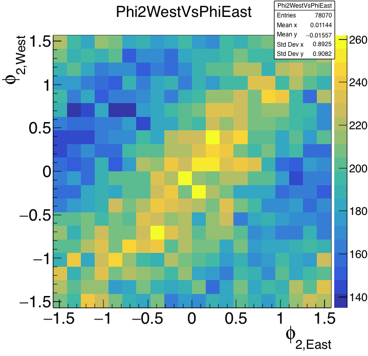
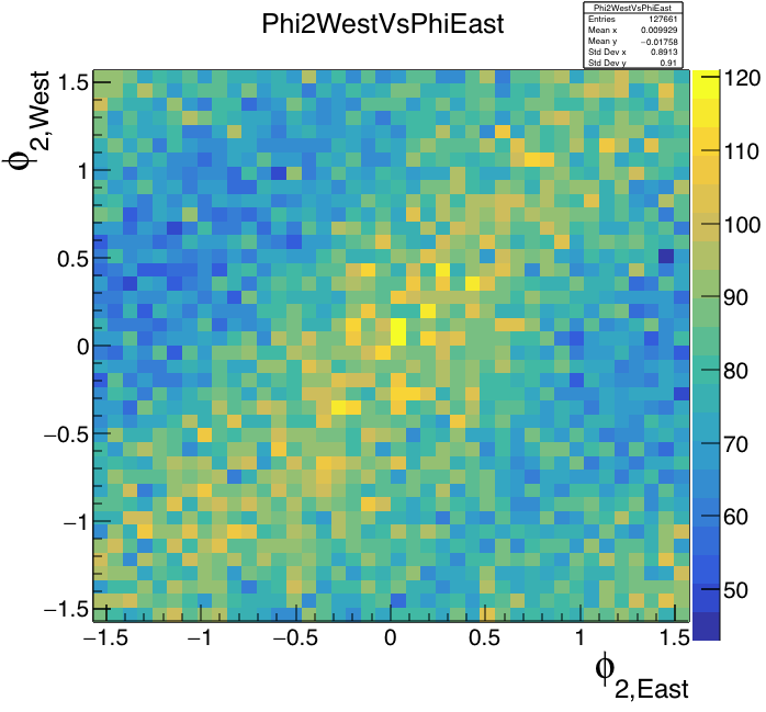
Figure 5: Left: Second-order event plane on the West side versus that on the East side, found with the Q-vector method in the EPD with tiles in the range 2<\eta<4. Mid-central (100<RefMult<200) events were used. Maximum allowed tile weight was 3 MPV1. Right plot: Finer binning with wider centrality cut (80<RefMult<250). The resolution is a little worse over this range, but more events makes finer binning possible, and a little nicer picture.
In the above plot, I used Max=3. Why? Because (in a limited search) that gave the best event plane resolution, as shown by the plot below:
.png)
Figure 6: Second-order event plane resolution for events with 100<RefMult<200, calculated with the simple formula above. Here, the value plotted at Max=8 actually corresponds to no limit.
We see that the event-plane resolution depends on the maximum weight cut-off, Max. The left-most point (Max=0.5) essentially treats the EPD as a hit/no-hit detector. The right-most point (plotted at Max=8, but actually corresponding to no software-imposed limit) weights according to ADC value with no cutoff, taking the tile's reported nMIP at face value, as it were. Even at these energies, it appears better to treat the EPD as a hit/no-hit detector than to blindly do nMIP-weighting. At least in this eta and centrality region, and with this particular algorithm.
The best resolution actually comes from a compromise approach, where the largest fluctuations are cut off, but we go beyond hit/no-hit. I had expected this. In fact, I had expected even a stronger dependence than the rather mild one shown in Figure 6.
Using Max=3, REP2=0.377. Again, this is not a spectacular number, but we haven't even started to optimize this thing yet. Eta weights, plane flattening, tuning, neural nets, innovation.... a lot ahead.
This comes from about 350 picoDst files, each holding about 1000 isobar collisions. Processing these 350K events takes about 2 wall-clock minutes on my mac. PicoDsts are definitely the way to go :-) Some global quantities first. (I suspect the small "spikes" in the RefMult plot are aliasing effects; I didn't look into it.)
Next, just a quick look at the ADCsum in the EPD versus other measures of centrality like RefMult (in the TPC) and ADCsum in the BBC. (I'll update this with finer bins if I get time.)
Next, with the Event Plane Detector, we want to look at.... the Event Plane!
Keep in mind that "the" Event Plane is not unambiguously defined. Though I have worked with this data only for a short time, it is abundantly clear to me that there will be LOTS of opportunity for innovation, tuning, and algorithm development to optimize our resolution. This will be exciting.
For the moment, I stay with the simplest Q-vector analysis.
Usually the sum in these equations is over N particles. However, we have 744 tiles (many having zero signal in any given event). I loop over these tiles (called StPicoEpdHits in the STAR framework).
The angle \phi_i is given by the center of the tile. (Aside: why does this drupal editor even have a "special character" menu, if it doesn't have Greek letters??)
For the weight, wi, I use
This approach is driven by the understanding that large fluctuations in energy loss due to the Landau tail can actually degrade the quality of a global quantity. Hence, the requirement that the weight not be greater than some value Max does not throw away valuable information, but rather throws away distorting fluctuations. Or, anyway, it can. The data can tell us.
I did a little messing around, but not much. I just wanted to see that it works, and then we "unblinded folks" will play with the data some more. To avoid the tiles where the fixed-target holder produces an anisotropy (this could be corrected for, but I just cut it out to be quick) I use tiles with pseudorapidity<4. The pseudorapidity \eta_i is given by a straight line that connects the primary vertex to the center of the tile. (As I've mentioned several times, a tile is not associated with some given \eta or \eta range. One must specify the primary vertex and the tile.)
The 2nd-order event plane was reconstructed separately on the East and West wheels, and the full event plane resolution may be evaluated through their correlation:
(Yes, Dr. Isaac Upsal admonished me that the prefactor of sqrt(2) is only an approximation and that I should find the root of some function a la Voloshin & Poskanzer. I'm being lazy.)
First, the correlation between East and West. Okay, it's not beautiful enough to hold a parade over, but it's the first look and to me it's beautiful. We will be able to improve greatly, I am sure.
Figure 5: Left: Second-order event plane on the West side versus that on the East side, found with the Q-vector method in the EPD with tiles in the range 2<\eta<4. Mid-central (100<RefMult<200) events were used. Maximum allowed tile weight was 3 MPV1. Right plot: Finer binning with wider centrality cut (80<RefMult<250). The resolution is a little worse over this range, but more events makes finer binning possible, and a little nicer picture.
In the above plot, I used Max=3. Why? Because (in a limited search) that gave the best event plane resolution, as shown by the plot below:
Figure 6: Second-order event plane resolution for events with 100<RefMult<200, calculated with the simple formula above. Here, the value plotted at Max=8 actually corresponds to no limit.
We see that the event-plane resolution depends on the maximum weight cut-off, Max. The left-most point (Max=0.5) essentially treats the EPD as a hit/no-hit detector. The right-most point (plotted at Max=8, but actually corresponding to no software-imposed limit) weights according to ADC value with no cutoff, taking the tile's reported nMIP at face value, as it were. Even at these energies, it appears better to treat the EPD as a hit/no-hit detector than to blindly do nMIP-weighting. At least in this eta and centrality region, and with this particular algorithm.
The best resolution actually comes from a compromise approach, where the largest fluctuations are cut off, but we go beyond hit/no-hit. I had expected this. In fact, I had expected even a stronger dependence than the rather mild one shown in Figure 6.
Using Max=3, REP2=0.377. Again, this is not a spectacular number, but we haven't even started to optimize this thing yet. Eta weights, plane flattening, tuning, neural nets, innovation.... a lot ahead.
»
- lisa's blog
- Login or register to post comments