Measuring a pseudorapidity distribution with the EPD
Updated on Fri, 2017-06-23 13:21. Originally created by lisa on 2017-06-22 21:31.
Measuring an eta distribution with the EPD seems almost laughably trivial. However, there is more involved than might be imagined, so this blog entry will illustrate a basic analysis. The data is the 54 GeV Au+Au data taken at the end of the 2017 run, with 1/8 of the EPD.
When I mention a hit/no-hit analysis below, that simply means incrementing the dN/deta distribution with unit weight, when a Tile's ADC value is above some threshold. I will try to convince you that a hit/no-hit analysis is not a good idea, at least for this data. (One can also imagine an "ADC-weighted" analysis, which is such a bad idea that I'm not even going to describe it.) For reference, we shall call the analysis I'm talking about here, the "Fit-based method" of extracting dN/deta.
I will illustrate the main points, but will also provide the code and more specific instructions for anyone who wants to use anything or more detail. I will put these pointers into [square brackets].
The data used
This analysis used 3.4M minimum bias events that had primary vertices. [Go here for details about data storage and macros used to make the histograms.]
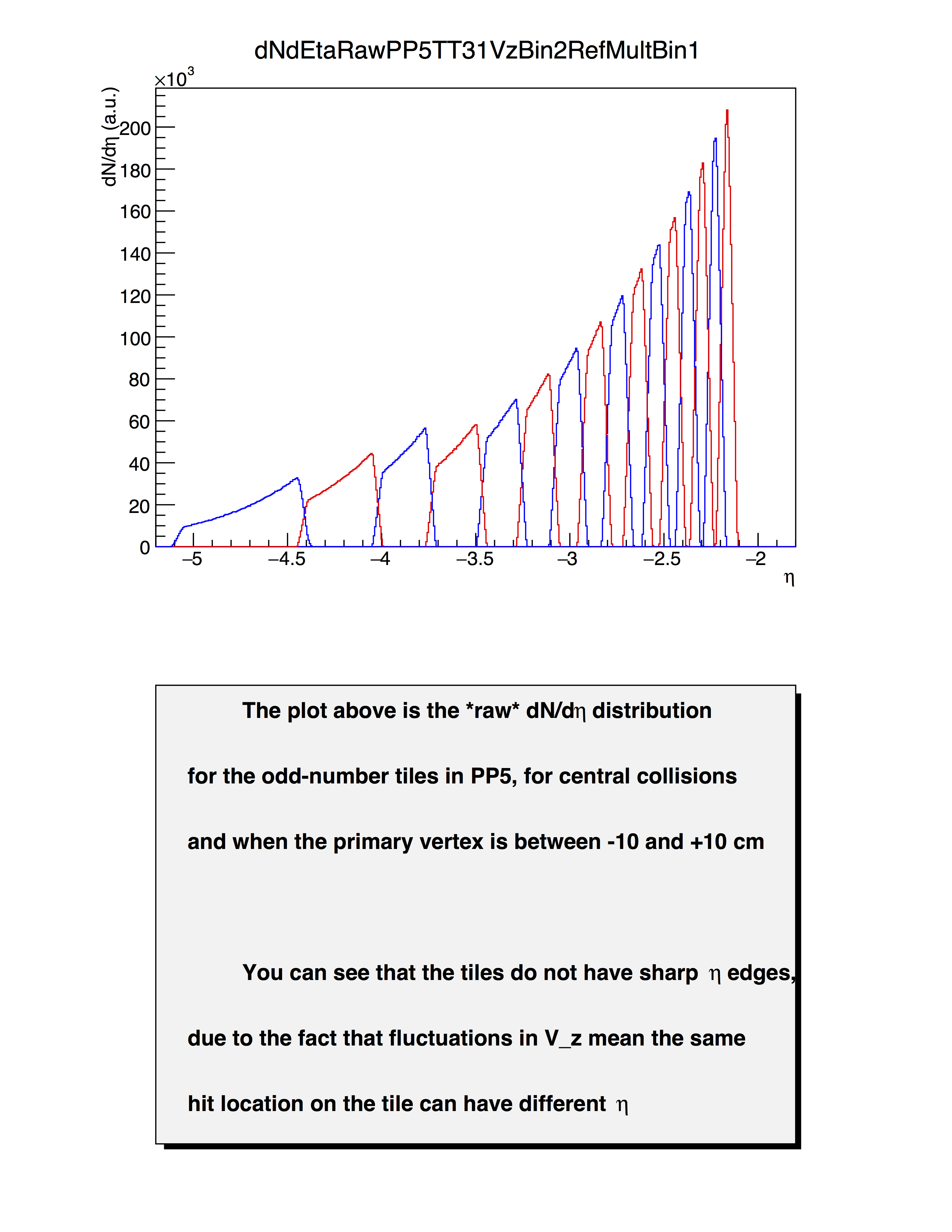
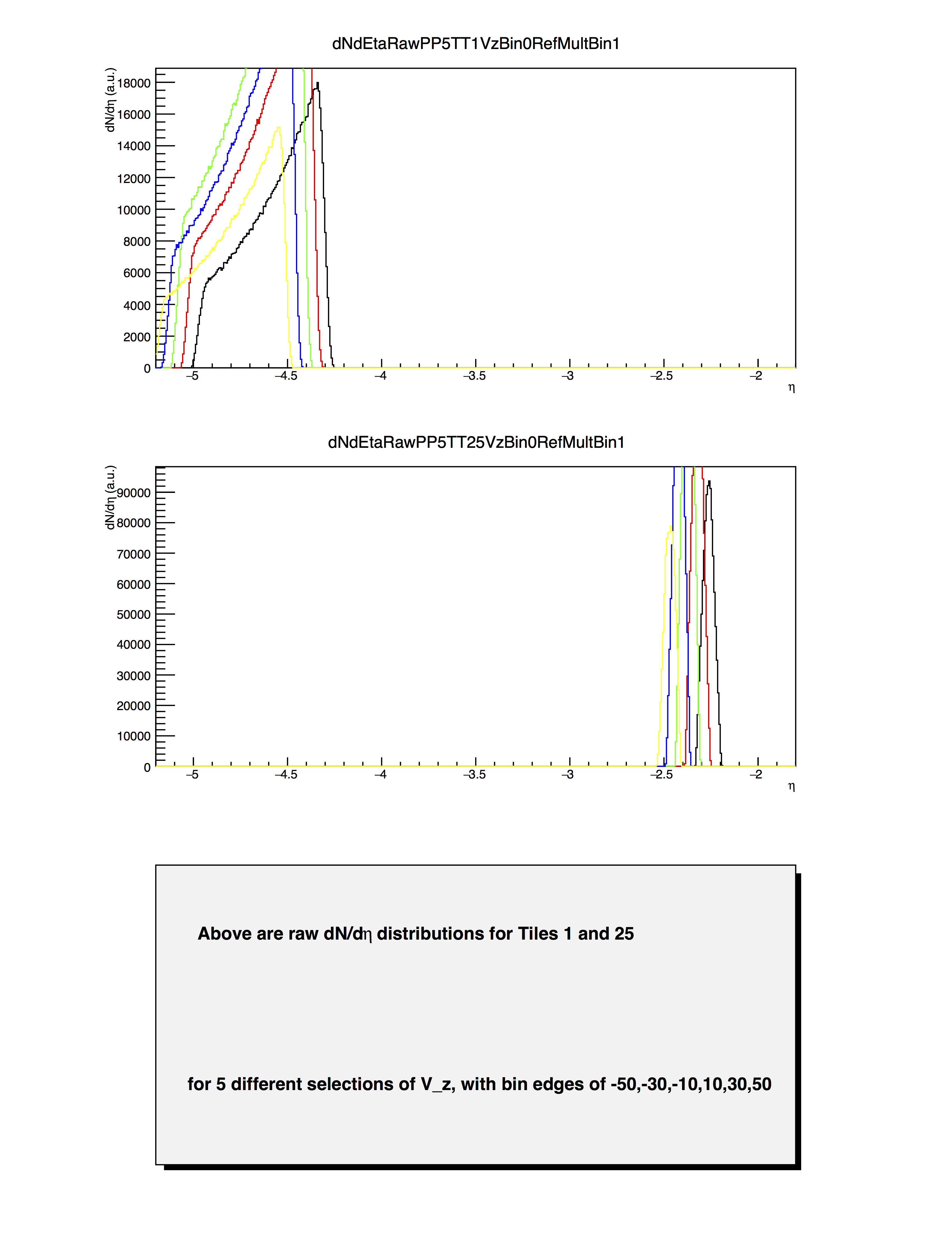
A Tile is struck-- what is eta?
The ADC distribution - with and without TDC cuts
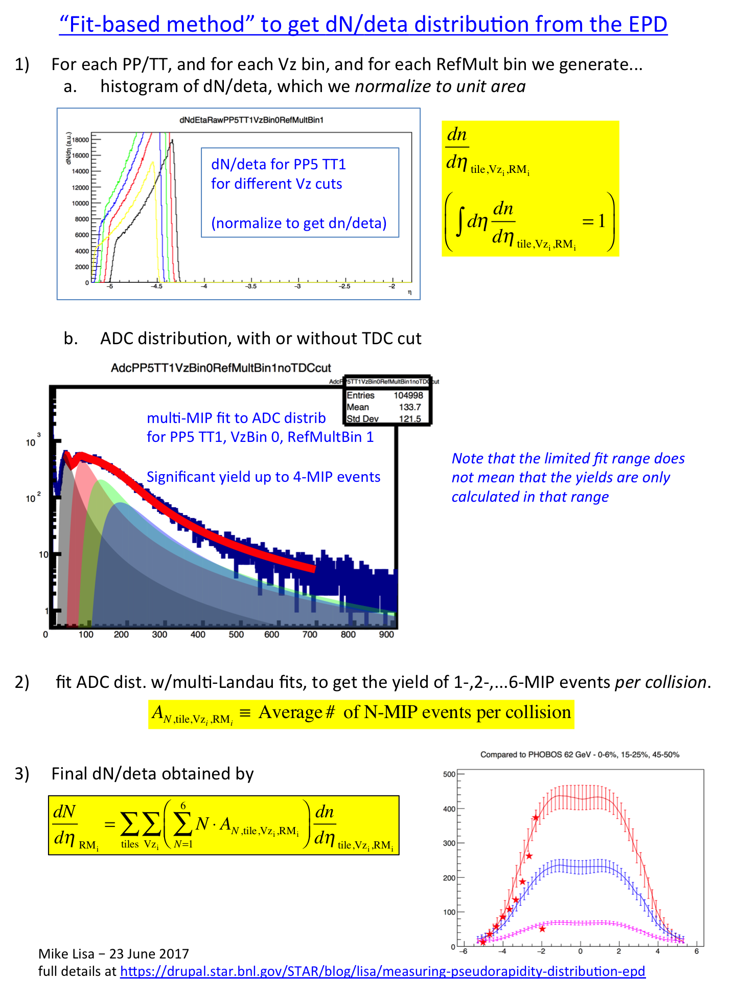
As I've illustrated before, in this data, we can have many particles pass through a Tile in a single event. In fact, most of the particles measured by a Tile are from multiple-MIP events. Hopefully that already makes it obvious that a hit/no-hit analysis is inappropriate. Rather, what must be done is to fit the ADC distribution and extract the 1-, 2-, 3-, ... N-MIP yields, and use these in a probabilistic way, to get the total number of particles. Importantly, this must be done for every tile and separately for every primary vertex position (range).
Naturally, it must also be done separately for any event cuts you use; this is clear from the plot below, which is the ADC distribution for PP6TT3 for 30<Vz<50. Blue is low RefMult and is high RefMult:
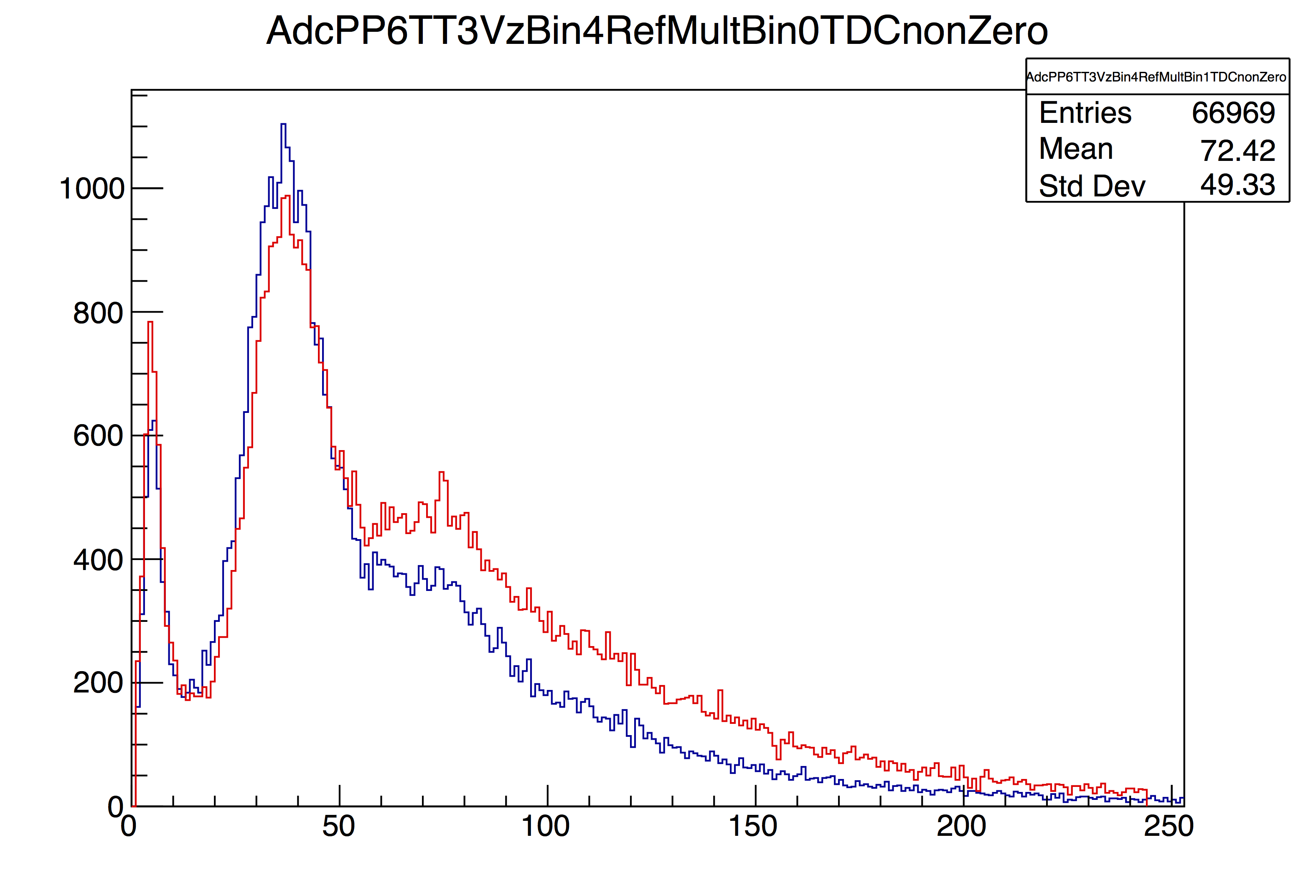
I have discussed the fact that a timing cut (on TAC) does a good job in removing out-of-time "noise" from the ADC distribution and that the TDC (which every channel has) tracks the TAC signal very nicely. Rosi has done a nice study showing that, for about 70% of our channels, TDC cuts remove the out-of-time stuff. I have verified this. Below, blue curves are with no TDC cut, and red are requiring non-zero TDC. Labels indicate whether the TDC for that channel will be useful.
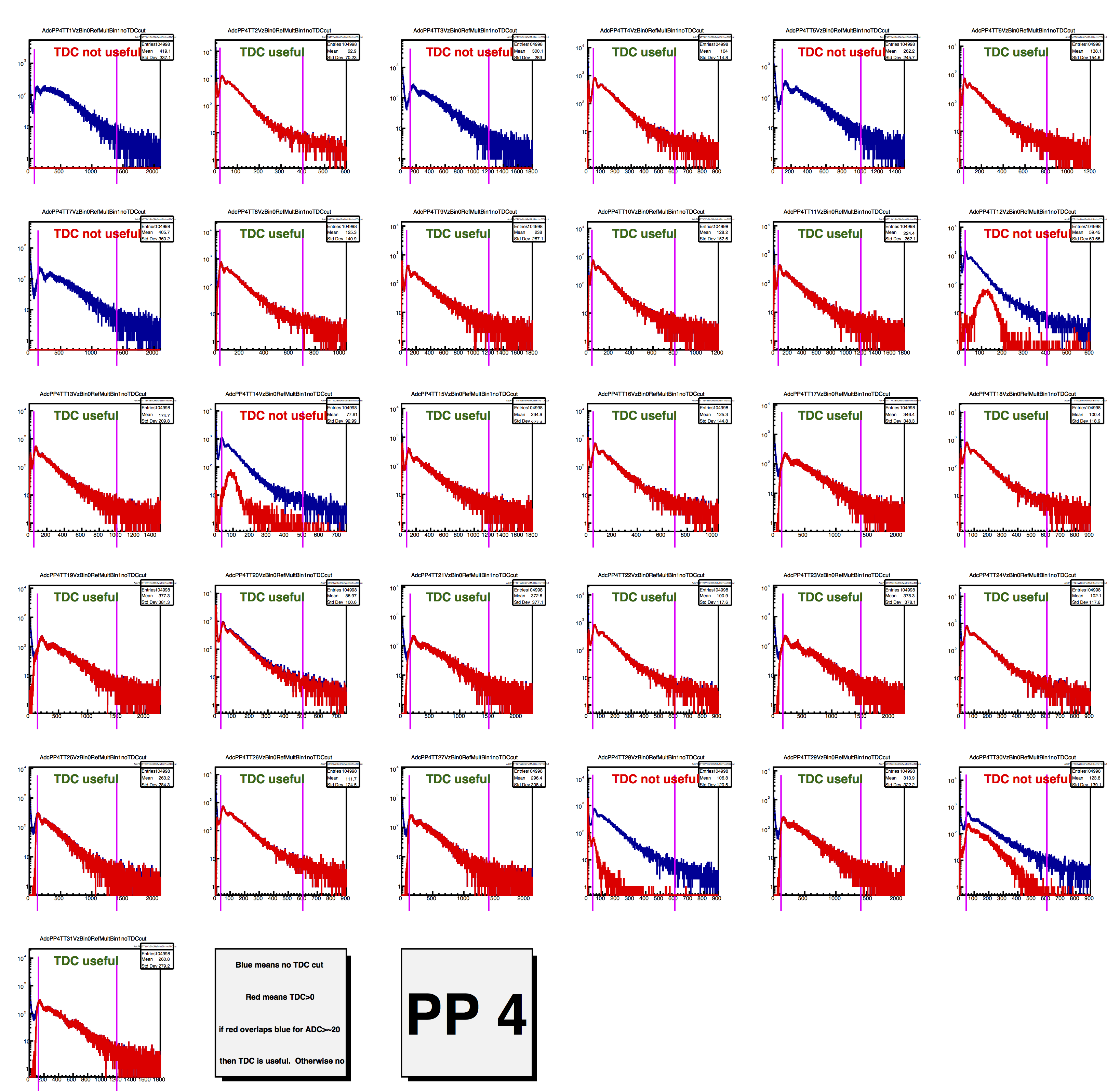
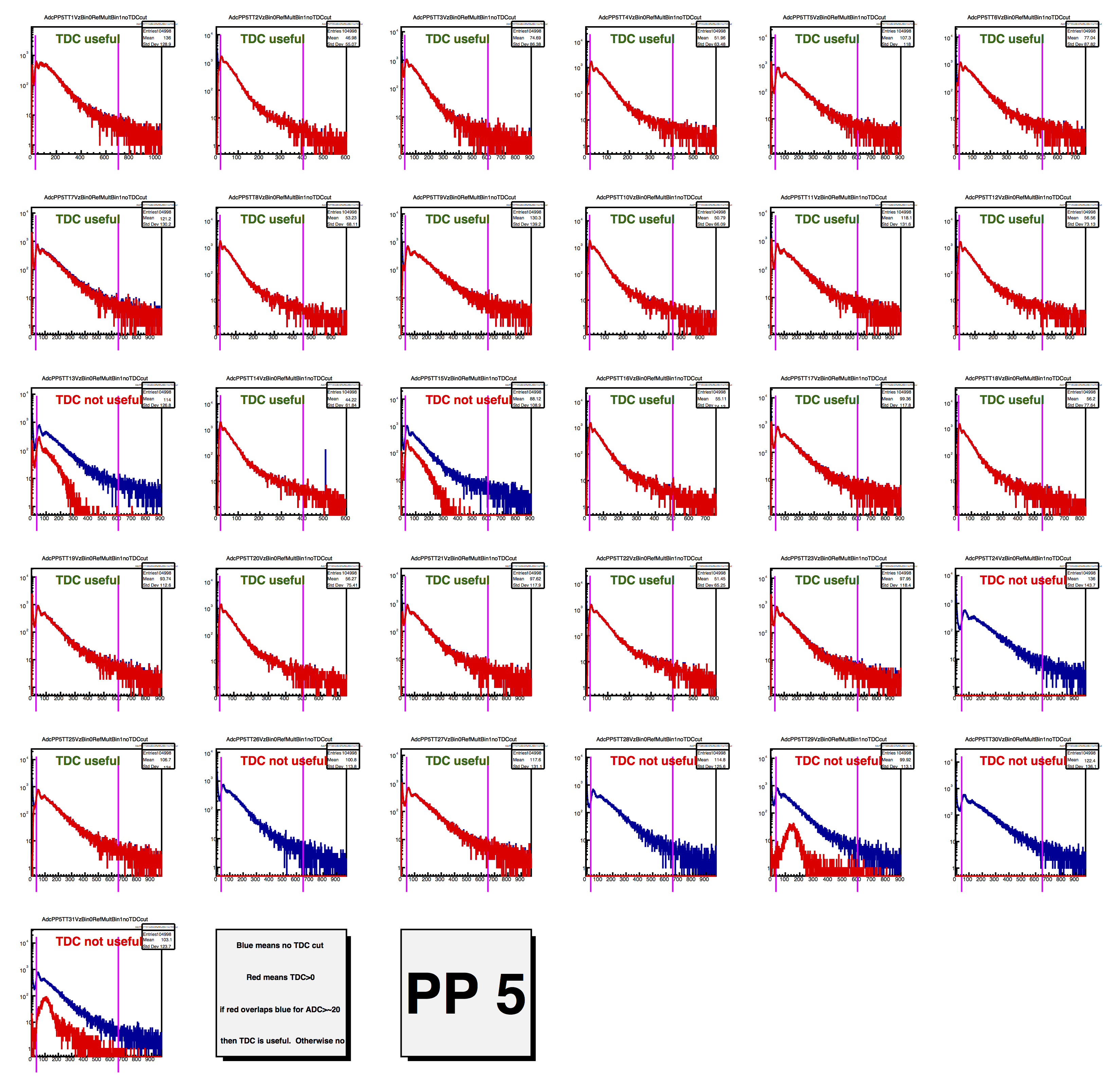
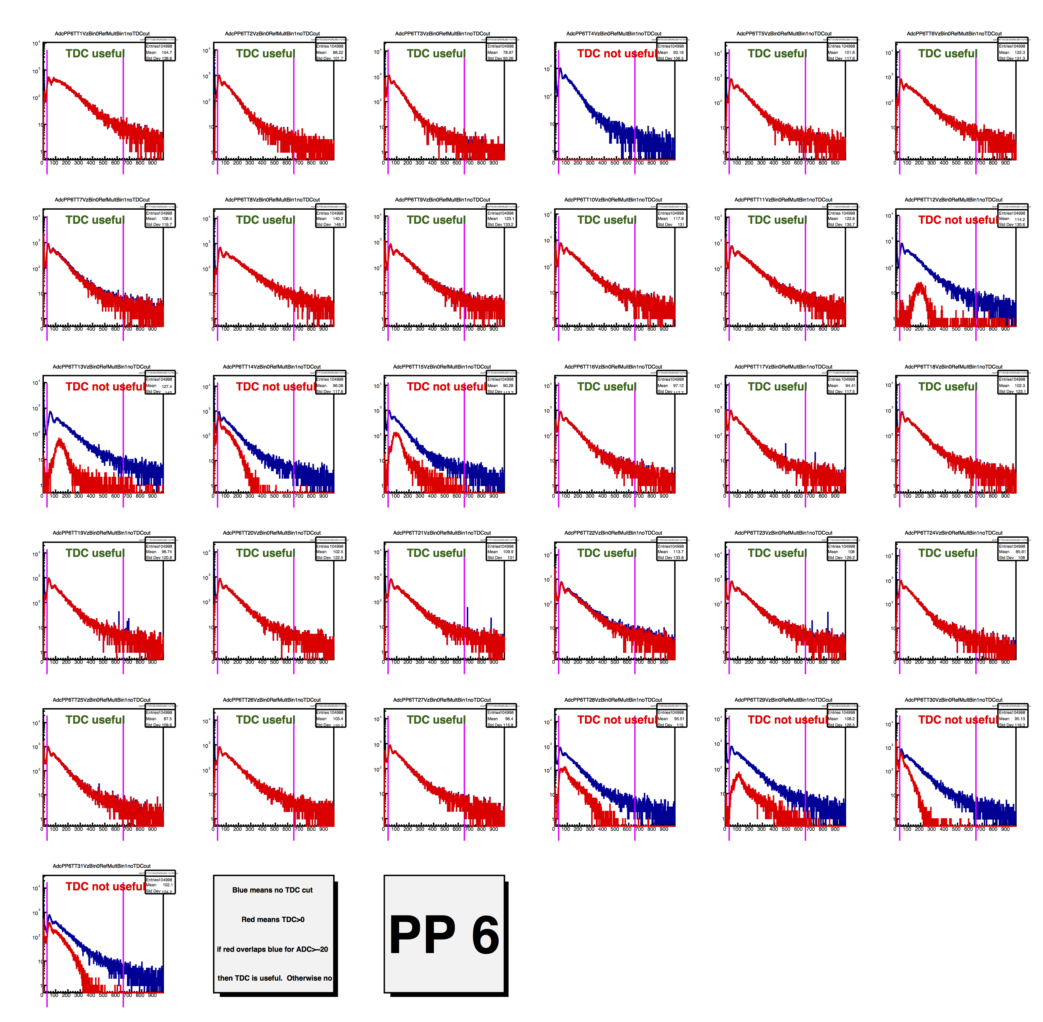
Those are small, I know. You can blow them up or look at the attached files for a full-resolution pdf file. Here is a blow-up of one of them:
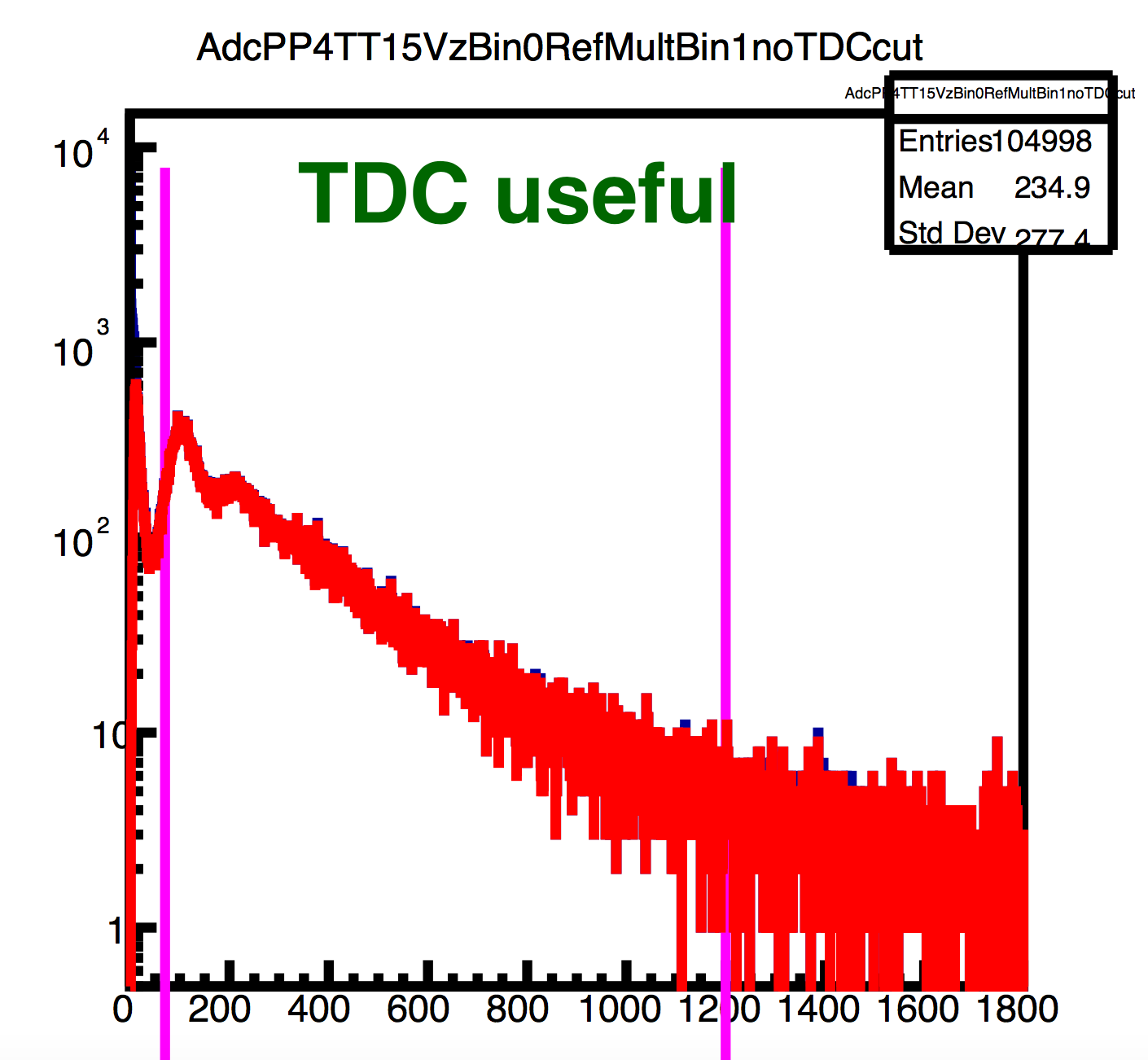
Since not every channel has a useful TDC, I decided to use no TDC cut, and simply fit a range of ADC values. This range is shown above by pink lines and is set individually for every tile.
Very important: this is not to be confused with a hit/no-hit analysis, where one might define a range (usually just a lower limit) that determines whether a Tile has been "hit." Such an analysis would be sensitive to this arbitrary range. The fit-based analysis I am discussing is not sensitive to the range used, so long as it is reasonable. It is fine if part of the "real signal" is outside of the fit range.
[Click for full-resolution pdf and for macro that made these pictures. A nice thing about the macro is that it has arrays identifying upper and lower ADC edges, as well as saying whether the channel has a useful TDC. I determined these by hand, so make use of it!]
Extracting the N-MIP yields
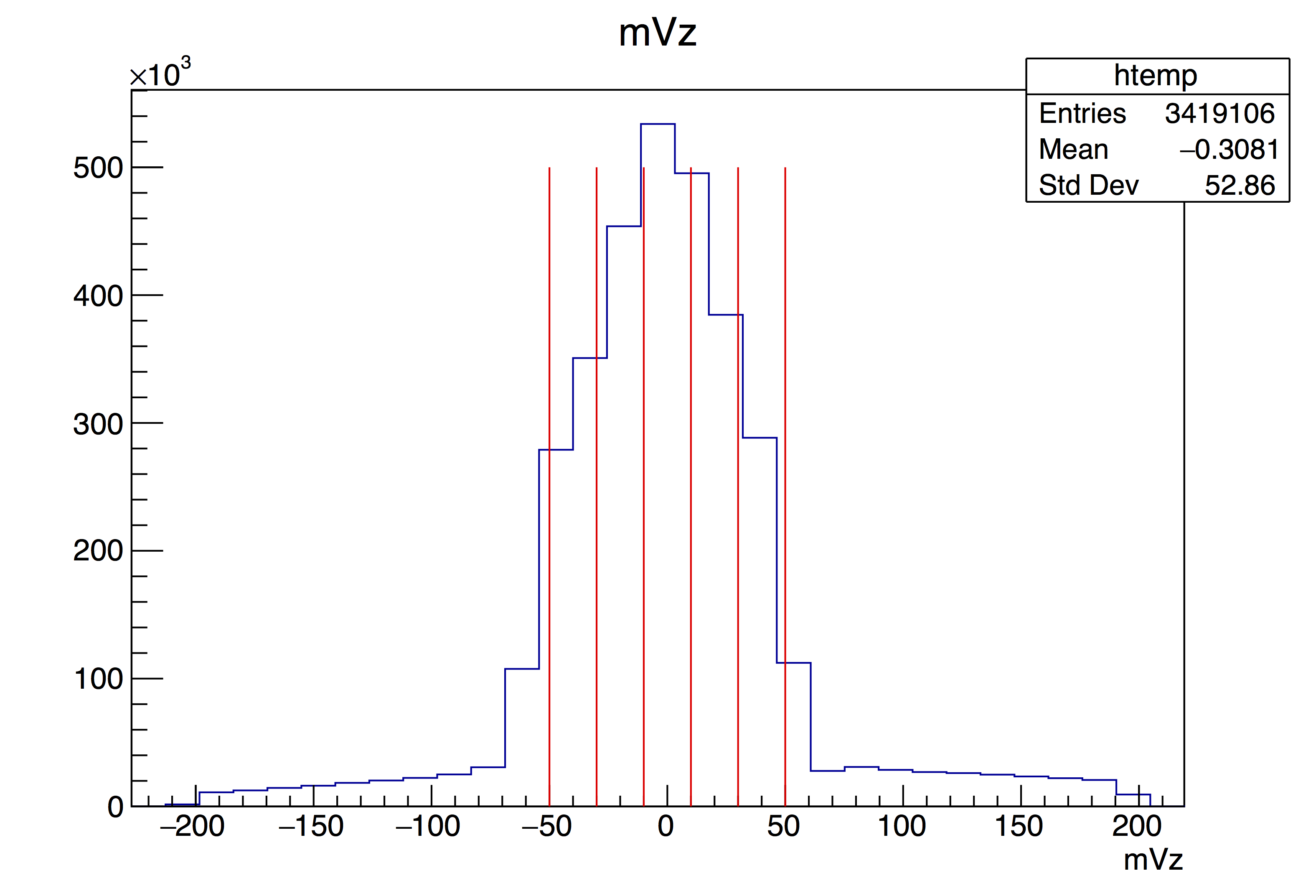
As mentioned above, these analyses must be performed for each cut in zVertex since (1) the eta distribution for a tile depends on Zvertex and (2) the ADC distribution will also depend on Zvertex. I have used 5 ranges in zVertex, 20-cm wide, for the range (-50 cm)<zVertex<(+50 cm). Furthermore, I have done the analysis for two ranges in RefMult. These are shown here:
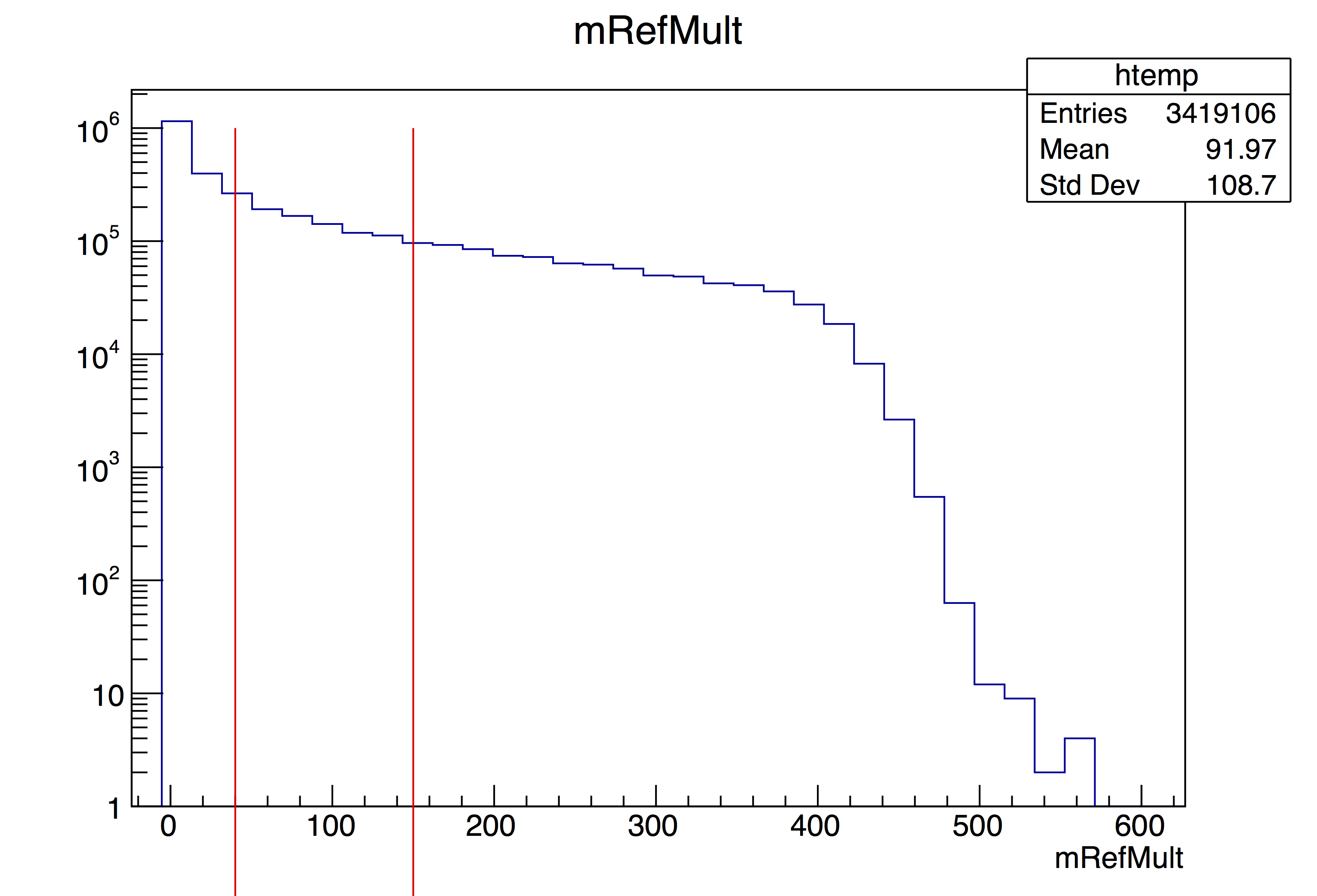
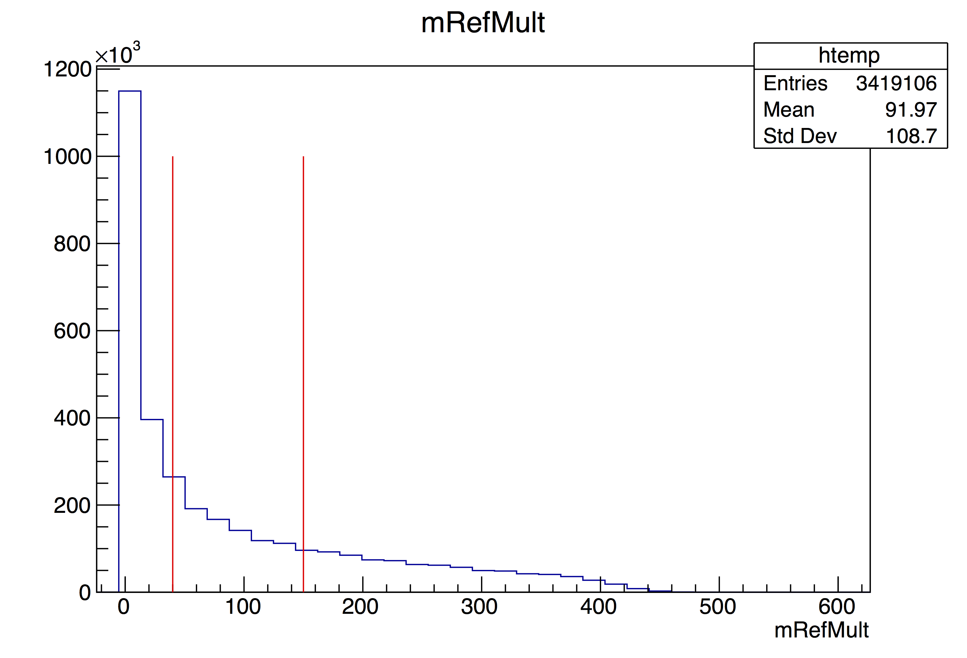
This means I had to make 3*31*5*2=930 ADC spectra, and fit them all. [Go here for more details on making the histograms to be fit, and here for some details on fitting them.]
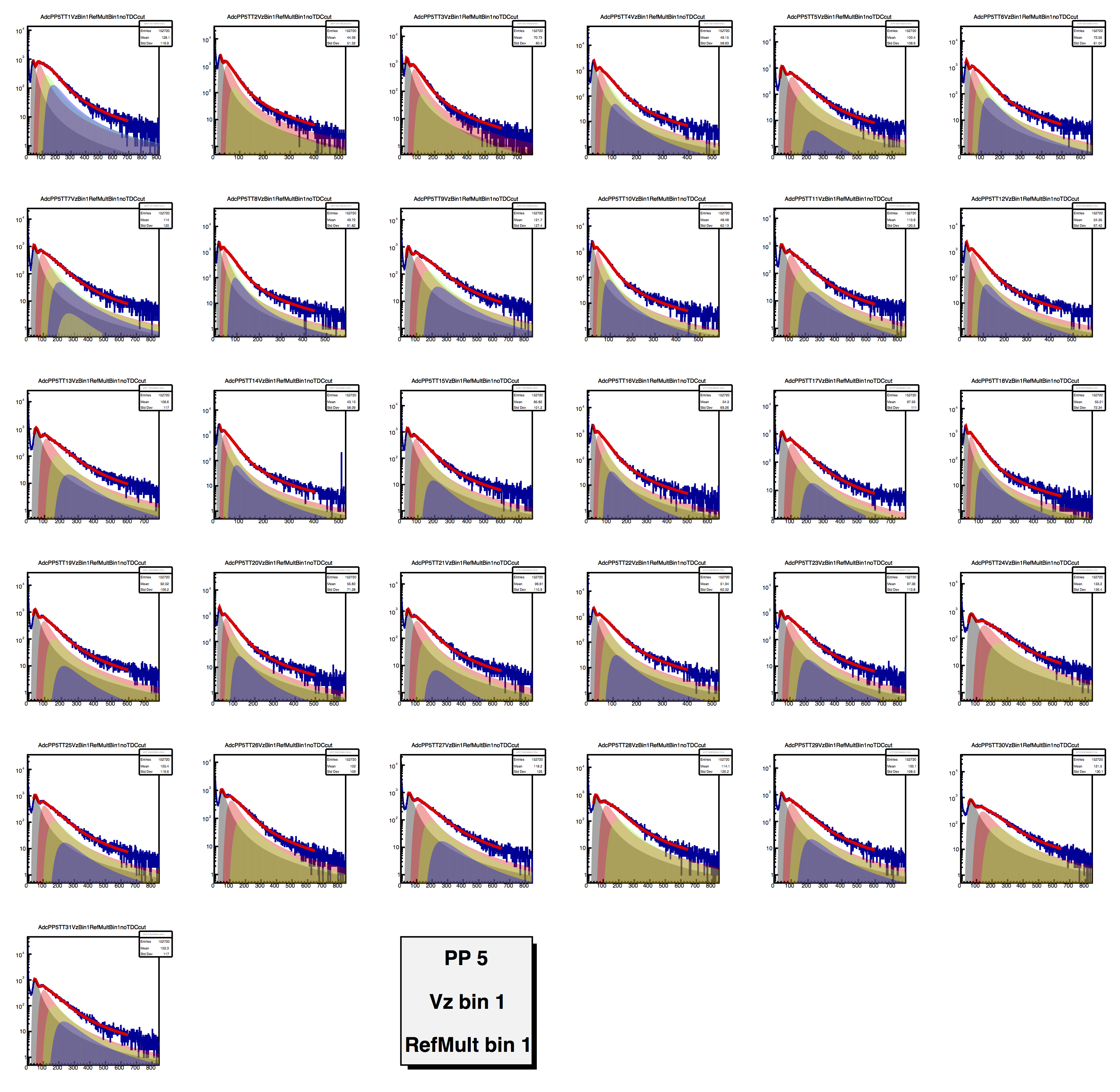
The fits were done automatically (of course), with the multi-MIP fitting method I discussed previously. Below see a small sample, for PP5, high RefMult, (-30 cm)<Vz<(-10 cm) Some fraction (3%?) of the fits gave "strange" fractions or didn't converge. I did not fix this, in this first look.
[A complete pdf of the fits is here.]
Putting it all together to get dN/deta:
For each tile (PP/TT), and each combination of Vz and RefMult selection, we now have
Don't sneer!!! It is a first analysis, and hopefully by now you see that it is not trivial.
What needs to be done, to get something final and publishable:
Here you find details that might not be of interest to the casual reader.
The data and the histograms:
The EPD data can be stored in STAR-independent TTrees (i.e. you can read them with just "vanilla" root) using the StEpdData structure. The StEpdMaker can produce these trees, and StEpd can read and process them. Rosi has extended the StEpdData structure to include some minimal non-EPD information, such as the primary vertex. The StEpdData object header is here. Rosi has recently stored the TTree files on a safe place on RCF, as she writes here. The many histograms one needs for this analysis are made by this macro.
Getting eta for a tile: Say Tile 8 on Position 4 on the East side is struck, and you want to increment an eta distribution. If the primary vertex is given by TVector3 VertexPos, then use the method TVector3 StEpdTile::RandomPointOnTile() as follows:
TVector3 straightLine = EPD->GetTile(4,8,-1)->RandomPointOnTile() - VertexPos; // EPD is an StEpd object
Double_t eta = straightLine.eta();
The StEpdTile::RandomPointOnTile() is the method Rosi uses to make the nice pictures of hit densities on the EPD wheel. (Though I caution that these are really "above-threshold event rates", not particle flux.)

Details on making the ADC spectra and fitting them:
You have to make a lot of histograms for this analysis. As mentioned above, you need 930 ADC spectra. You also need 930 eta distributions (one for each multiplicity, zVertex, and Tile). Producing the histograms to fit is described above. The fits are summed convoluted Landau distributions, which I've discussed before. The macro to fit the histogram file is here.
A warning: This macro fits the 31 Tiles in one Vz bin in one RefMult bin. This is all that my laptop can handle before root crashes, because the size of the process grows to 15 GB!!! So, I had to run the thing over and over, with a trivial shell script you can find here.
Plots of all fits are here, and the fit parameters of all of the fits can be found here.
A one-page primer on how to combine the information to get the final distribution:
When I mention a hit/no-hit analysis below, that simply means incrementing the dN/deta distribution with unit weight, when a Tile's ADC value is above some threshold. I will try to convince you that a hit/no-hit analysis is not a good idea, at least for this data. (One can also imagine an "ADC-weighted" analysis, which is such a bad idea that I'm not even going to describe it.) For reference, we shall call the analysis I'm talking about here, the "Fit-based method" of extracting dN/deta.
I will illustrate the main points, but will also provide the code and more specific instructions for anyone who wants to use anything or more detail. I will put these pointers into [square brackets].
The data used
This analysis used 3.4M minimum bias events that had primary vertices. [Go here for details about data storage and macros used to make the histograms.]
A Tile is struck-- what is eta?
- We will assume that the charged particles travel in straight lines (they don't) and further assume that they originate at the primary vertex (some don't).
- We will not assume that a Tile was struck at its center, but will assume a uniform probability of being hit. (This will not be strictly correct.)
- Eta is then dictated by the slope of the line connecting a random point on the tile with the primary vertex. [If you want more detail, go here.]
The ADC distribution - with and without TDC cuts
As I've illustrated before, in this data, we can have many particles pass through a Tile in a single event. In fact, most of the particles measured by a Tile are from multiple-MIP events. Hopefully that already makes it obvious that a hit/no-hit analysis is inappropriate. Rather, what must be done is to fit the ADC distribution and extract the 1-, 2-, 3-, ... N-MIP yields, and use these in a probabilistic way, to get the total number of particles. Importantly, this must be done for every tile and separately for every primary vertex position (range).
Naturally, it must also be done separately for any event cuts you use; this is clear from the plot below, which is the ADC distribution for PP6TT3 for 30<Vz<50. Blue is low RefMult and is high RefMult:
I have discussed the fact that a timing cut (on TAC) does a good job in removing out-of-time "noise" from the ADC distribution and that the TDC (which every channel has) tracks the TAC signal very nicely. Rosi has done a nice study showing that, for about 70% of our channels, TDC cuts remove the out-of-time stuff. I have verified this. Below, blue curves are with no TDC cut, and red are requiring non-zero TDC. Labels indicate whether the TDC for that channel will be useful.
Those are small, I know. You can blow them up or look at the attached files for a full-resolution pdf file. Here is a blow-up of one of them:
Since not every channel has a useful TDC, I decided to use no TDC cut, and simply fit a range of ADC values. This range is shown above by pink lines and is set individually for every tile.
Very important: this is not to be confused with a hit/no-hit analysis, where one might define a range (usually just a lower limit) that determines whether a Tile has been "hit." Such an analysis would be sensitive to this arbitrary range. The fit-based analysis I am discussing is not sensitive to the range used, so long as it is reasonable. It is fine if part of the "real signal" is outside of the fit range.
[Click for full-resolution pdf and for macro that made these pictures. A nice thing about the macro is that it has arrays identifying upper and lower ADC edges, as well as saying whether the channel has a useful TDC. I determined these by hand, so make use of it!]
Extracting the N-MIP yields
As mentioned above, these analyses must be performed for each cut in zVertex since (1) the eta distribution for a tile depends on Zvertex and (2) the ADC distribution will also depend on Zvertex. I have used 5 ranges in zVertex, 20-cm wide, for the range (-50 cm)<zVertex<(+50 cm). Furthermore, I have done the analysis for two ranges in RefMult. These are shown here:
This means I had to make 3*31*5*2=930 ADC spectra, and fit them all. [Go here for more details on making the histograms to be fit, and here for some details on fitting them.]
The fits were done automatically (of course), with the multi-MIP fitting method I discussed previously. Below see a small sample, for PP5, high RefMult, (-30 cm)<Vz<(-10 cm) Some fraction (3%?) of the fits gave "strange" fractions or didn't converge. I did not fix this, in this first look.
[A complete pdf of the fits is here.]
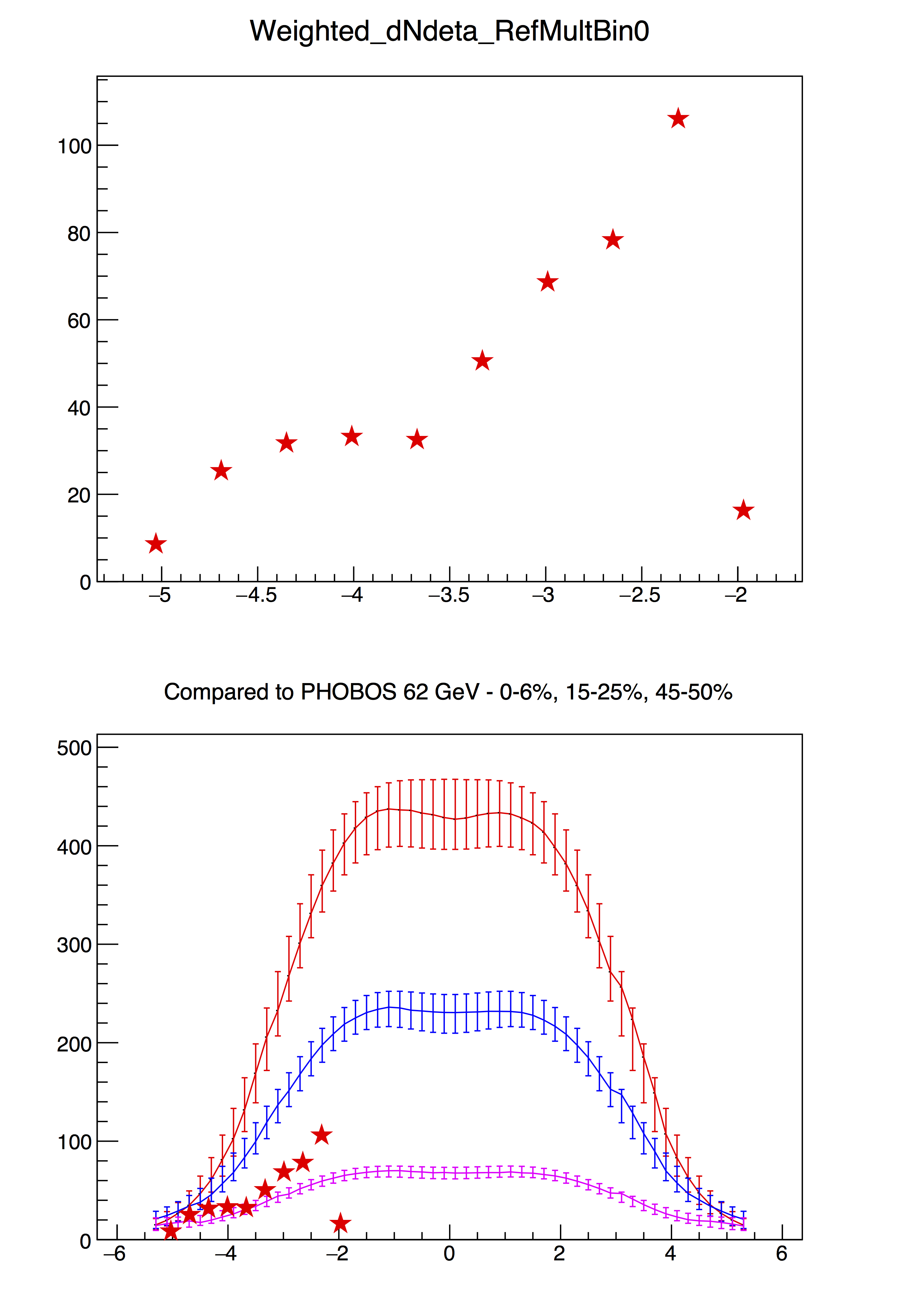
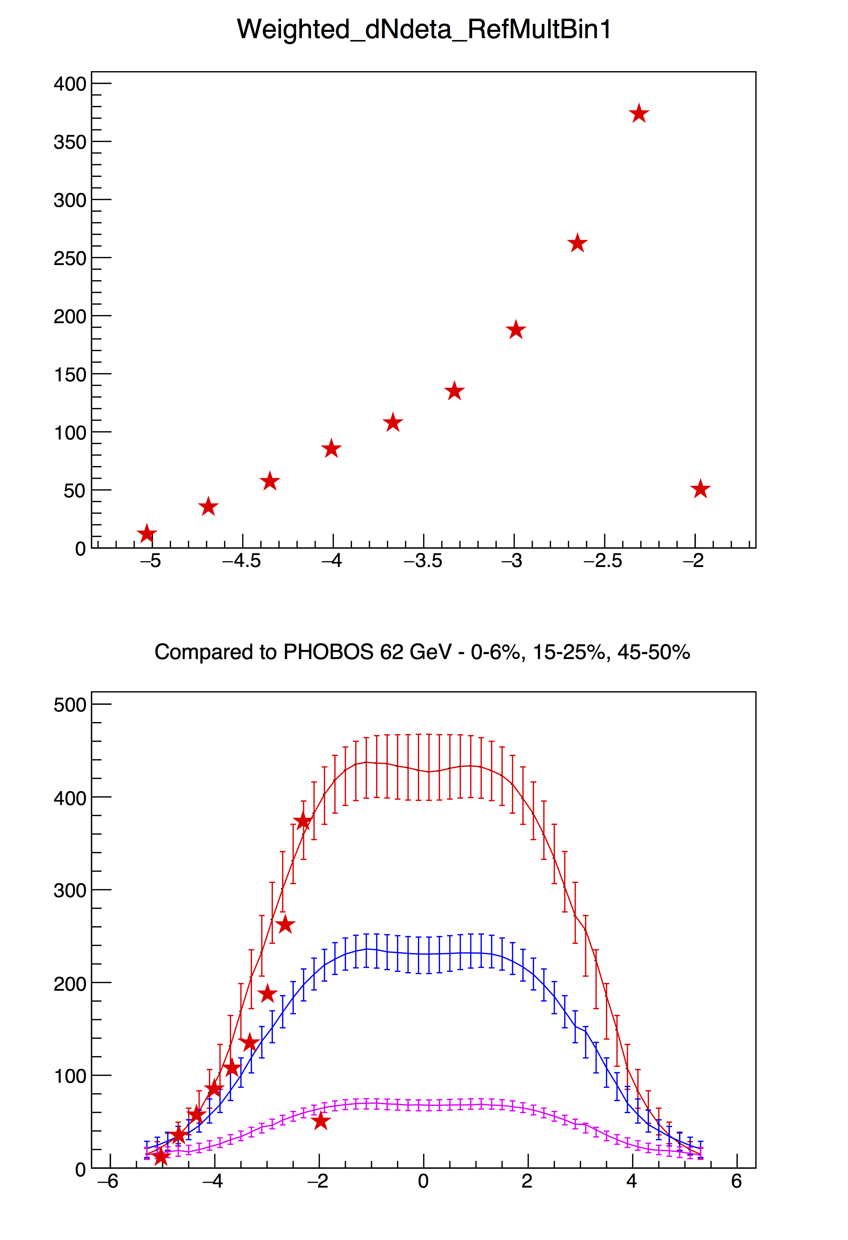
Putting it all together to get dN/deta:
For each tile (PP/TT), and each combination of Vz and RefMult selection, we now have
- the shape of the dN/deta distribution (normalized to unity)
- 1-, 2-, 3-, 4-, 5-, and 6-MIP yields (which is used to normalize)
Don't sneer!!! It is a first analysis, and hopefully by now you see that it is not trivial.
What needs to be done, to get something final and publishable:
- Calculate errorbars. This can be done using the uncertainties on the N-MIP yields that come from the fits.
- Take care about the multi-MIP fits that go wonky. Shouldn't be too hard to identify and simply "help the fits" along a bit
- Efficiency correction. For this we need Sam's work with Geant.
- We know that the straight-line approximation is incorrect-- these particles travel in a helix. This must be accounted for, and it requires an assumption of the pT distribution. Sam will have to tell us this
- Hanseul points out that the assumption of uniform hit probability over the face of a Tile is only an approximation. The real probability distribution is of course determined by the eta distribution itself. This means we would have to do a kind of "iterative" correction to fix this approximation, using the data itself to correct itself. It should not be too hard, but details have to be worked out.
- Probably we should use finer Vz bins. Mine are 20-cm wide here. 5 cm might be better.
- We should choose RefMult bins in a reasonable way. I just did two here, as an example
Here you find details that might not be of interest to the casual reader.
The data and the histograms:
The EPD data can be stored in STAR-independent TTrees (i.e. you can read them with just "vanilla" root) using the StEpdData structure. The StEpdMaker can produce these trees, and StEpd can read and process them. Rosi has extended the StEpdData structure to include some minimal non-EPD information, such as the primary vertex. The StEpdData object header is here. Rosi has recently stored the TTree files on a safe place on RCF, as she writes here. The many histograms one needs for this analysis are made by this macro.
Getting eta for a tile: Say Tile 8 on Position 4 on the East side is struck, and you want to increment an eta distribution. If the primary vertex is given by TVector3 VertexPos, then use the method TVector3 StEpdTile::RandomPointOnTile() as follows:
TVector3 straightLine = EPD->GetTile(4,8,-1)->RandomPointOnTile() - VertexPos; // EPD is an StEpd object
Double_t eta = straightLine.eta();
The StEpdTile::RandomPointOnTile() is the method Rosi uses to make the nice pictures of hit densities on the EPD wheel. (Though I caution that these are really "above-threshold event rates", not particle flux.)
(PositionOfTileCenter - VertexPosition
Details on making the ADC spectra and fitting them:
You have to make a lot of histograms for this analysis. As mentioned above, you need 930 ADC spectra. You also need 930 eta distributions (one for each multiplicity, zVertex, and Tile). Producing the histograms to fit is described above. The fits are summed convoluted Landau distributions, which I've discussed before. The macro to fit the histogram file is here.
A warning: This macro fits the 31 Tiles in one Vz bin in one RefMult bin. This is all that my laptop can handle before root crashes, because the size of the process grows to 15 GB!!! So, I had to run the thing over and over, with a trivial shell script you can find here.
Plots of all fits are here, and the fit parameters of all of the fits can be found here.
A one-page primer on how to combine the information to get the final distribution:
»
- lisa's blog
- Login or register to post comments