Publications
Publications:
- Measurements of the Z0/γ⁎ cross section and transverse single spin asymmetry in 510 GeV p + p collisions, Phys. Lett. B 854 (2024) 138715
- Longitudinal and transverse spin transfer to Lambda and anti-Lambda hyperons in polarized p+p collisions at sqrt{s} = 200 GeV. Phys. Rev. D 109 (2024) 12004
- Azimuthal transverse single-spin asymmetries of inclusive jets and identified hadrons within jets from polarized pp collisions at sqrt{s} = 200 GeV. Phys. Rev. D 106 (2022) 72010
-
Evidence for Nonlinear Gluon Effects in QCD and Their Mass Number Dependence at STAR. Phys. Rev. Lett. 129 (2022) 092501
-
Longitudinal double-spin asymmetry for inclusive jet and dijet production in polarized proton collisions at sqrt(s) = 510 GeV. Phys. Rev. D 105 (2022) 92011
-
Longitudinal double-spin asymmetry for inclusive jet and dijet production in polarized proton collisions at sqrt(s) = 200 GeV. Phys. Rev. D 103 (2021) L091103
- Comparison of transverse single-spin asymmetries for forward pi0 production in polarized pp, pAl and pAu collisions at nucleon pair c.m. energy sqrt(sNN) =200 GeV Phys. Rev. D 103 (2021) 72005
- Measurement of transverse single-spin asymmetries of pi0 and electromagnetic jets at forward rapidity in 200 and 500 GeV transversely polarized proton-proton collisions Phys. Rev. D 103 (2021) 92009
- Measurements of W and Z/gamma Cross Section and Cross-Section Ratios in p+p Collisions at RHIC. Phys. Rev. D 103 (2021) 012001
- Longitudinal double spin asymmetry for inclusive jet and dijet production in pp collisions at sqrt(s) = 510 GeV. Phys. Rev. D 100 (2019) 052005
- Measurement of the longitudinal spin asymmetries for weak boson production in proton-proton collisions at sqrt(s) = 510 GeV. Phys. Rev. D 99 (2019) 051102
- Transverse spin transfer to Lambda and anti-Lambda hyperons in polarized proton-proton collisions at sqrt(s)=200 GeV. Phys. Rev. D 98 (2018) 091103
- Improved measurement of the longitudinal spin transfer to Lambda and Anti-Lambda hyperons in polarized proton-proton collisions at sqrt(s) = 200 GeV. Phys. Rev. D 98 (2018) 112009
- Longitudinal Double-Spin Asymmetries for Dijet Production at Intermediate Pseudorapidity in Polarized pp Collisions at sqrt(s) = 200 GeV. Phys. Rev. D 98 (2018) 032011
- Longitudinal double-spin asymmetries for pi0s in the forward direction for 510 GeV polarized pp collisions. Phys. Rev. D 98 (2018) 032013
- Transverse spin-dependent azimuthal correlations of charged pion pairs measured in p+p collisions at sqrt(s)=500 GeV. Phys. Lett. B 780 (2018) 332-339
- Azimuthal transverse single-spin asymmetries of inclusive jets and charged pions within jets from polarized-proton collisions at sqrt(s) = 500 GeV. Phys. Rev. D 97 (2018) 32004
- Measurement of the cross section and longitudinal double-spin asymmetry for di-jet production in polarized p+p collisions at sqrt(s) = 200 GeV. Phys. Rev. D 95 (2017) 71103
- Measurement of the transverse single-spin asymmetry in p+p -> W±/Z0 at RHIC. Phys. Rev. Lett. 116 (2016) 132301
- Observation of Transverse Spin-Dependent Azimuthal Correlations of Charged Pion Pairs in p+p at sqrt(s)=200 GeV. Phys. Rev. Lett. 115 (2015) 242501
- Precision Measurement of the Longitudinal Double-spin Asymmetry for Inclusive Jet Production in Polarized Proton Collisions at sqrt(s) = 200 GeV. Phys. Rev. Lett. 115 (2015) 92002
- Measurement of longitudinal spin asymmetries for weak boson production in polarized proton-proton collisions at RHIC. Phys. Rev. Lett. 113 (2014) 72301
- J/psi polarization in p+p collisions at sqrt(s) = 200 GeV in STAR. Phys. Lett. B 739 (2014) 180
- Neutral pion cross section and spin asymmetries at intermediate pseudorapidity in polarized proton collisions at sqrt(s)=200 GeV. Phys. Rev. D 89 (2014) 12001
- Single Spin Asymmetry A_N in Polarized Proton-Proton Elastic Scattering at sqrt(s)=200 GeV. Phys. Lett. B 719 (2013) 62
- Transverse Single-Spin Asymmetry and Cross-Section for pi0 and eta Mesons at Large Feynman-x in Polarized p+p Collisions at sqrt(s) = 200 GeV Phys. Rev. D 86 (2012) 51101
- Longitudinal and transverse spin asymmetries for inclusive jet production at mid-rapidity in polarized p+p collisions at sqrt(s)=200 GeV. Phys. Rev. D 86 (2012) 32006
- Measurement of the W->e+nu and Z->e+e Production Cross Sections at Mid-rapidity in Proton-Proton Collisions at sqrt(s) = 500 GeV. Phys. Rev. D 85 (2012) 92010
- Measurement of the parity-violating longitudinal single-spin asymmetry for W-boson production in polarized proton-proton collisions at sqrt(s) = 500 GeV. Phys. Rev. Lett. 106 (2011) 62002
- Longitudinal double-spin asymmetry and cross section for inclusive neutral pion production at midrapidity in polarized proton collisions at sqrt(s) = 200 GeV. Phys. Rev. D 80 (2009) 111108
- Longitudinal Spin Transfer to Lambda and anti-Lambda Hyperons in Polarized Proton-Proton Collisions at sqrt(s) = 200 GeV. Phys. Rev. D 80 (2009) 111102
- Forward Neutral Pion Transverse Single Spin Asymmetries in p+p Collisions at sqrt(s)=200 GeV. Phys. Rev. Lett. 101 (2008) 222001
- Longitudinal double-spin asymmetry for inclusive jet production in p+p collisions at sqrt(s)=200 GeV. Phys. Rev. Lett. 100 (2008) 232003
- Measurement of Transverse Single-Spin Asymmetries for Di-Jet Production in Proton-Proton Collisions at sqrt(s)= 200 GeV. Phys. Rev. Lett. 99 (2007) 142003
- Longitudinal Double-Spin Asymmetry and Cross Section for Inclusive Jet Production in Polarized Proton Collisions at sqrt(s) = 200 GeV. Phys. Rev. Lett. 97 (2006) 252001
- Cross Sections and Transverse Single-Spin Asymmetries in Forward Neutral Pion Production from Proton Collisions at sqrt(s)= 200 GeV. Phys. Rev. Lett. 92 (2004) 171801
2006 FPD inclusive neutral pion AN link
2006 inclusive jet paper (ALL, AN, ATT, and AΣ). link
- PWGC paper preview presentation 7/11/2008
- STAR Publications and Data page
Charged pion cross section and ALL link
- PWGC paper preview presentation 9/5/2008
2005 Lamda spin transfer paper link
2005 BEMC inclusive neutral pion paper (ALL, z frag.) link
- PWGC paper preview presentation 2/24/2009
- STAR Publications and Data page
2009 W AL link
2009 W and Z cross section link
2006 FPD neutral pion and η cross section and AN link
2006 EEMC inclusive neutral pion cross section, ALL, and AN link
2012 W AL link
2005 Charged Pion
Paper Proposal
Cross section and longitudinal double-spin asymmetry for inclusive charged pion production in polarized proton collisions at sqrt(s) = 200 GeV
Proposed Target Journal
Phys. Rev. Lett.
Principal Authors
A. Kocoloski, L. Ruan, B. Surrow, Y. Xu, Z. Xu
Abstract
We report an extension in transverse momentum to 15 GeV/c for the differential cross section and a first measurement of the longitudinal double-spin asymmetry A_{LL} for inclusive midrapidity charged pion production in polarized proton collisions at sqrt(s) = 200 GeV. The pi-/pi+ ratio shows significant p_{T} dependence from unity at low p_{T} to 0.83±0.01(stat)±0.04(syst) at high p_{T}, an experimental signature of significant valence quark contribution. The next-to-leading order perturbative QCD models incorporating flavor dependence in the fragmentation functions can describe the cross sections and the isospin asymmetry. The charged pion A_{LL} data covering 2 < pT < 13 GeV/c disfavor a large polarized gluon distribution in the proton and provide the first glimpse of a direction of future measurements. The predicted A_{LL} difference in the positively and negatively charged pions can be tested in future RHIC data.
Summary
In summary, we report the differential cross section and longitudinal double-spin asymmetry A_{LL} for inclusive charged pion production at midrapidity in polarized proton collisions at sqrt(s) = 200 GeV. The pion cross sections were determined up to p_{T} = 15 GeV/c and are described by NLO pQCD evaluations over 7 orders of magnitude. The asymmetries A_{LL} cover 2 < p_{T} < 13 GeV/c. They are consistent with NLO pQCD calculations utilizing polarized quark and gluon distributions from inclusive DIS analyses and disfavor large positive values of gluon polarization in the polarized nucleon.
Proposed Figures
Figure 1: “Technical” or “instrumental” figure on the use of a jet patch trigger for this analysis. Final graphics are still to be determined. The left panel shows the minimum-bias and triggered distributions obtained from PYTHIA simulations and used to correct the measured pion spectra. The right panel plots the mean fraction of the jet momentum carried by associated (R=0.4) charged pions in the case of jets that fired the trigger (black filled squares) and jets opposite trigger jets (red open squares). The inset shows the ($\eta$, $\phi$) distribution of charged pions relative to the trigger jet in the data.

Figure 2: Transverse momentum spectra for charged pions at midrapidity ($\left|{y}\right| < 0.5$) (a) and comparison of data to DSS prediction versus $p_{T}$ (b). (c) shows ratio of π-/π+ data compared to DSS and AKK predictions.

Figure 3: The longitudinal double-spin asymmetry $A_{LL}$ in $\vec{p} + \vec{p} \rightarrow \pi^{+/-} + X$ at $\sqrt{s}=200 GeV$ versus pion $p_{T}$. The uncertainties on the data points are statistical. The gray bars indicate the total point-to-point systematic uncertainty, and the curves show predictions based on parameterizations of gluon polarization from global analyses.

Supporting Documentation
Asymmetry :: Cross Section
2005 Dijet
Supporting documentation on the 2005 Dijet Paper, targetted for PRDRC
Title: Dijet production in proton-proton collisions at sqrt(s) = 200 GeV
PAs: Matthew Walker, Joseph Seele, Bernd Surrow
Abstract:
We report the first STAR measurement of the differential cross section for midrapidity dijet production in proton-proton collisions at sqrt{s}=200 GeV. The cross section data cover invariant mass $20<M<117 GeV/c^2 and agree well with next-to-leading order perturbative QCD calculations.
Summary:
In summary, a measurement of the cross section for dijet production at midrapidity with the STAR detector at RHIC is reported over the invariant mass range 20 < M < 117 (GeV/c^2). Good agreement with a NLO pQCD calculation after applying a correction for underlying event and hadronization is observed. This agreement motivates the use of pQCD calculations for comparisons to spin observables, such as the longitudinal double-helicity asymmetry, A_{LL}, which can be used to obtain constraints on the polarized parton distributions in the proton. Increased detector acceptance and luminosity in future data sets make this measurement appealing. Furthermore, the framework is already in place to incorporate a dijet A_{LL} into a global fit.
Proposed Figures (order may differ in paper):
Fig. 1 Data Simulation Comparison (pdf attached)
Caption: (Left panel top) The comparison of data (red) and simulation (blue) yields as a function of invariant mass. The simulation normalization has been set so the integrals of data and simulation are the same over the range 20 to 86 GeV/c^2 in invariant mass. (Left panel bottom) The ratio of data to simulation as a function of invariant mass. (Center panels) The comparison of data and simulation and the ratio of data to simulation as a function ofeta_{34} = \frac{\eta_3 + \eta_4}{2}. (Right panels) The comparison of data and simulation and the ratio of data to simulation as a function of cos{\theta^*}.

Fig. 2 Cross Section (pdf attached)
Caption: (top panel) Differential cross section for p + p \rightarrow \textrm{jet} + \textrm{jet} + X at \sqrt{s} = 200 GeV vs dijet invariant mass for a jet cone radius of 0.4. The data in each bin are marked with the black line depicting the bin width and statistical uncertainties as a vertical line. Systematic uncertainties for the data are shown in yellow bands. The single hashed bands are the NLO calculation from de Florian. with scale uncertainties. The double hashed bands are the same calculation with the hadronization and underlying event correction applied. (bottom panel) Comparison of theory and data. The data are compared to the theory calculation with hadronization and underlying event correction. The same statistical and systematic uncertainty bands are shown along with the scale uncertainties.
Fig. 2 version 2 (pdf attached)
.png)
Fig. 3 Event Display (not final):
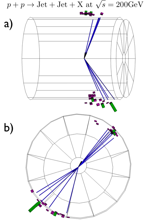
Fig. 4 Lego plots (not final):
.png)
2006 di-jet Sivers PRL paper
Measurement of Transverse Single-Spin Asymmetries for Di-Jet Production in Proton-Proton Collisions at sqrt(s) of 200 GeV
Target Journal: PRL
Principal Authors (PA): J.Balewski, I.Qattan, and S.Vigdor
Abstract+summary+figures (ver 1.2) : link to protected/spin area
Status:
presented to PWGC on December 01,
pwg approved to request GPC, Decmeber 14,
GPC phone conference , January 4
- Draft of the PRL paper version 1.2 (posted November 16, 2006)
- Comments/suggestions for ver 1.2
* from Carl , received on Nov 16
* from Hal ,received on Nov 27
* - Revised ver 1.3 (ps) , posted December 12,
- Akio,Les: I guess the biggest question I had was east BEMC "problem" and your measurement on Nov 30
The 2% of the off-line data have be reanalyzed with the new (electron based) BTOW gains to verify the previous conclusions hold, as posted on Issam's summary page, spin-hn, on January 11, 2007
- Akio,Les: I guess the biggest question I had was east BEMC "problem" and your measurement on Nov 30
- Comments from GPC are listed below
- Peter J., Jan 4, 2007
- Revised draft ver 2.0 (January 29, 2007)
- Comments from Mike, Feb 2,2006, below
Mike M., Feb 02, 2007
<pre>Hi all,
some brief comments after reading the newest draft (v2).
1) Overall, I really like the way the first page reads -- well done.
2) I think it's lacking a crisp explanation of why online jets are used instead of offline, perhaps I missed it.
3) I think that Figure 2 should clearly be labeled as "Simulation". It's in the caption, but the minute the figure gets clipped into a presentation the caption (and that info) are gone.
4) I would prefer the use of "Fast Monte Carlo" instead of "toy model," for various reasons. First, anyone in particle physics will probably understand that Fast MC implies not doing full simulation/ reconstruction, but a quick smearing. Furthermore, there's enough info in the MC that you believe the results, whereas the phrase "toy" makes it sound otherwise. Second, anybody outside of particle physics won't know the difference between a fast MC and a full slow simulation.
5) Personally I find Figure 3 fairly confusing, especially when dumped to BW. I realize this comes down to matters of taste, but I personally prefer to show the model calculations as binned histograms (TH1::Draw("hist")). The markers are in my mind too easily confused with the data (given that this is really 6 plots). Further, the "hist" option will clearly show that the models were binned the same as the data, and makes a nice distinction between data/theory. By a clever choice of line styles, you can probably even make this fairly clear in BW.
6) In Figure 3 and in the text, would it be possible to use some english to differentiate between A_N(>pi) vs A_N(<pi). Maybe introduce the phrases "quark-like" and "gluon-like"? If you can find a smooth way, it would sure make the p4 text smoother, and give some intuition to fig 3.
I realize it'sa little tricky because Fig3b is kind of an orphan. Do you really need it? They're straight lines , and you could quote 4 numbers in the text in a single sentence, even cutting down on some space. Then you could have a "quark-like" left panel and a "gluon- like" right panel.
But, again, I really like the draft.
-Mike
Peter J., Jan 4, 2007
Hi GPC and PAs,Here are some first comments on the paper draft:
(i) physics intro, 1st para: I find the physics intro to be a bit confusing. I looked briefly at refs [6,7] (Brodsky et al and Collins). Within my distinctly limited understanding of them I don't think the last sentence of the first paragraph is accurate, and the main physics point of interest in this measurement is missed.
Evidently, the SSA arises due to interference of left- and right-handed quark polarization states, and thus is sensitive to chiral symmertry breaking. If correct, this is important and should be featured prominently in the intro.
On the other hand, I am confused by the various claims about factorization in this process. Brodsky et al claim that the process cannot be factored into PDF and FF, while Collins claims that factorization holds but then derives a pdf $f_{1T}^\perp$ whose sign is opposite for DIS and DY (eq 3), i.e. a pdf whose value is process-dependent, which doesn't sound to me like factorization. The only thing I know for sure is that I am confused on this point and could use some guidance. I suspect that most non-experts will be similarly confused. The physics intro should be precise and clear about what the theory says.
(ii) p 1 left col 2nd para bottom: what is the specific relevance to this measurement of the inclusive jet cross section being described by (factorized) pQCD? I guess if it didn't work for the inclusive yields one could stop immediately. Is that the only point to be made here? Can one say more about constraints on PDFs and FFs?
(iii) p 1 right col line 9: I know nothing about Siberian snakes. What are the limits on possible non-vertical polarization states?
(iv) End of that para: give errors on polarization: 59\pm{xx}\% (57\pm{yy}\%).
(v) jet reconstruction: nowhere do you actually describe what "jet reconstruction" you do. P 2 left col line 6 talks about "jet clusters at level 2" and the caption of Fig 1 talks about "full jet reconstrcution" but the reader is left hanging about how a jet is actually defined. Is there some peak-finding with a cut-off radius, or what? I know that you use EMC energy only but the non-expert reader will not know what this implies, i.e. all of the EMC energy plus perhaps 30% of the charged hadronic energy, with some charged-track dispersion in the magnetic field that is not corrected for. You need a couple of paragraphs defining the jet finding used for the analysis and giving its comparison to full jet reco, justifying why this technique is adequate for this measurement (there is currently some of that later in the text but it should be consolidated).
(vi) Fig 1d: why only 2% of the data? I think I know the answer: that's what was reconstructed at the time you were in the thick of this analysis, but evidently more has been done in the meantime. Not usable?
(vii) p 2 left col middle: I printed the paper in B&W and don't see the 6-fold L0 peaks in fig 1a. Am I missing them?
(viii) p 2 right col 2nd para: the "favoring" of qg vs gg at forward vs midrapidity is qualitative. Can this be made quantitative, e.g using PYTHIA? What is the magnitude of the variation of the two contributions?
(ix) p 2 right col middle: "while we away the time-consuming replay of the full dataset including TPC..." is a STAR detail of little interest to others, and has a limited shelf-life. I suggest simply describing what was done, saying that this rapid analysis technique (in contrast to full jet reco) is sufficient for present purposes.
(x) Fig 1b and discussion of tails in p2 right col bottom: "might reflect moderately hard gluon emission" is weak. Can this be studied with a model calculation? But I also find it confusing because I don't know how the jet finding was done. Hard gluon emission will generate an acoplanarity only if it pushes some of the energy flow out of the jet cone, otherwise momentum is conserved. So I suspect that this tail depends on how the jet is defined. Needs more discussion.
I also wonder about tails being generated by the combination of relatively low multiplicity in low energy jets and only partial jet reco (EM plus ~30% hadronic, with some funny spread in the latter due to the field). Could unfavorable, perhaps rare, fluctuations in charged vs neutral pions generate such apparent tails which are not present for full jet reco? Perhaps a model study would help here. Anyway, the toy model in which you just fit with a Gaussian with an exponential seems inadequate - can you do a more meaningful study based on PYTHIA or HERWIG?
(xi) p 3 left col top: is there a jet energy dependence to <kT^2>? More generally, the distribution shown in Fig 1d goes out to ~50 GeV if I jack it up by eye by a factor 50. Can you make a few coarse energy bins to look at the dependence of the asymmetry on jet energy? You say somewhere that you expect the ET dependence of the Sivers effect to be small, but surely it would be good to test this.
(xii) definitions of A_N and r_\pm (eq 1 and 2): it's late in the evening and I am a bit tired, but frankly these formulas are not speaking to me at the moment. A_N is defined as the ratio of ratios, which is OK, but I am not getting the purpose of the sqrt. There are too many +- and -+ subscripts and zeta>pi vs zeta<pi which are hard to distinguish. Can you find a more transparent notation, or explain the structure of the definitions a bit better?
That's all for now. I didn't read the last third as carefully, I'll do that next time.
Hope these are helpful, talk to you tomorrow.
Peter
Inclusive Jet Definition at STAR
Target Journal: PRD
Principal Authors: M. Miller, J. Balewski, R. Fatemi, A. Kocoloski, F. Simon, J. Sowinski, D. Staszak, B. Surrow, S. Trentalange, S. Vigdor
Abstract: We present a detailed study of jet reconstruction in the STAR detector at RHIC. Jets are reconstructed via a mid-point cone clustering of charged particle tracks and electromagnetic showers. We provide a detailed summary of the definition of the jet energy scale, primarily the \textit{in situ} calibration of the calorimeter, a precise definition of the jet algorithm, and various correction factors derived from Monte Carlo studies. Finally, we measure the inclusive jet cross section at $\sqrt{s}$ = 200 GeV, corrected for non-perturbative effects, and compare to several NLO calculations. We find good agreement between data and theory, and note that the non-perturbative corrections are as large as the scale dependence of the calculation.
BEMC Calibration
This page is intended to provide documentation of how I arrived at the numbers and figures relevant to the BEMC calibration quoted in the paper. Data and macros can be found athttp://deltag5.lns.mit.edu/~kocolosk/protected/long_jet_paper/
If you want to reproduce these plots, you're probably best off just downloading the whole directory. Here's a tarball:
http://deltag5.lns.mit.edu/~kocolosk/protected/long_jet_paper/bemcCalibration.tar
2003
Nothing to see here just yet. I asked Alex about the availability of the data and was told that they used the last dAu combined production.2004
Run 4 BTOW CalibrationNevents = 20-57 M. Run 4 is funny because we've reproduced P05ia since I did my analysis, so the old query I used isn't really valid anymore. I took these numbers from Jamie's page at
http://www.star.bnl.gov/protected/common/common2004/trigger2004/200gev/sums_emc.txt
The 20M number is the total number of trigId==15007 events. These are what we used for the MIP calibration, but we also applied centrality and vertex cuts that aren't reflected in that number. The number is also complicated by the warning not to use minbias triggers from productionLow || Mid || High before 5042040, which I did not heed (not sure if we knew about the problem at the time). For the electrons we required trigId!=15203, which if I take all-bTid15203 from that link gives me 57.2M events.
No attempt has been made to figure out exactly what fraction of these data was actually analyzed in my jobs. In Run 5 that number was 94%, here I've just taken it to be 100%.
Nmips = 1.4 x 10^{6}. This is the number of entries in the "mH0" histogram in 2004_mips.root
Nelectrons = 1.5 x 10^{6} makeElectronCounts.C The reason we have Nmips ~= Nelectrons is that the electron sample dropped the refMult and vertex cuts and took some triggered data as well. Specifically, we used trigId==15007 for the MIPs and trigId!=15203 for the electrons.
Figure 2a: makeMipFigures.C
Figure 4a: makeElectronFigure2.C
Figure 5: makeGainsFigure.C
Note that in each case you'll have to download the ROOT files required by the macro and put them in the same directory.
2005
Run 5 BTOW CalibrationNevents = 57M. This one is a bit tricky, as I never saved a tree with all the events I looked at. Here's how I arrived at the number. I used a catalog query
get_file_list.pl -cond 'production=P05if,filetype=daq_reco_mudst,storage=HPSS,filename~physics,sanity=1,tpc=1,emc=1' -keys 'sum(sanity),sum(events),sum(size),grp(trgsetupname)'to get number of files and events for each trgsetupname I used in the calibration (ppProduction || ppProductionMinBias || ppTransProduction). The query returned a total of 73716 files in HPSS. I did save my original filelists, and when I cat them together I find that I analyzed about 94% of available files (69297 to be exact). The event sample from catalog was 60.8 M events, and I just multiplied that number by the percentage of analyzed files. This doesn't reflect the |vz|<30 cut that was applied to the MIP study.
Nmips = 4.3 x 10^{6} This is the number of entries in "h" in 2005_mips.root. All the cuts from Run 5 BTOW Calibration had already been applied. You might have noticed that this number is much larger than the number of MIPs in Run 4. The reason for this is that in Run 4 we used only minbias (trigId == 15007) and we also applied a centrality cut of 60-100% (refMult<57). In addition, it's quite a lot harder to find an isolated track in a AuAu event versus a pp event, and Run 5 had a 3/4 barrel instead of just 1/2.
Nelectrons = 0.4 x 10^{6} makeElectronCounts.C applies all the cuts and spits out the final counts for 2004 and 2005.
Figure 2b: makeMipFigures.C
Figure 4b: makeElectronFigure2.C
Figure 5: makeGainsFigure.C
Figure 8: makeElectronFigure3.C