Offline Software
Embedding
Welcome to the STAR Embedding Pages!
Embedding data are generally used in STAR experiments for detector acceptance & reconstruction efficiency study. In general, the efficiency depends on running conditions, particle types, particle kinematics, and offline software versions. In principle, each physics analysis will need to formulate its own embedding requests by providing all the above relevant information. In STAR Collaboration, the embedding team is assigned to process those embedding requests and provide these embedding data, you can find out how the embedding team works in the Embedding structure page.
Over the past years, lots of embedding requests from different PWG's have been processed by the embedding team, please find the list in STAR Simulations Requests interface. If you want to look at some of these data, but do not know where these data are stored, please go to this page. If you can not find similar embedding request, you need to formulate your own embedding request for your particular study, please go to this page for more information about how to formulate an embedding request.
Please subscribe to the embedding mailing list if you are interested with embedding discussion: Starembd-l@lists.bnl.gov
And please join our weekly embedding meeting : https://drupal.star.bnl.gov/STAR/node/65992
Finding existing embedding data
Embedding data were produced for each embedding request in the STAR Simulations Request page.
Normally, they will be stored in RCF NFS disks for a while for end users to do their analysis.
However, NFS disk space is very limited, and we have new requests constantly, the data will be finally moved
from disks to HPSS for permanent storage on tape, but they can be restaged to disk for analysis later.
In order to find the existing embedding either on disks or in HPSS. Please follow the procedures below:
1) Find the request ID of a particular request that you are interested in, in the STAR Simulations Request page.
You can use the "Search" box at the top right of this page. Once you find the entry, look at the 'Request History' tab for more information, usually the original NFS data directory (when the data was first produced) can be found there.
2) Currently, the RCF NFS disks for embedding data are /star/data105, /star/embed and /star/data18.
For the data directories of each request, please logon to RCF, look at '/star/data105', '/star/embed' or '/star/data18' to see whether the following directories exist:
/star/data105/embedding/${Trigger set name}/${Embeded Particle}_${fSet}_${RequestID}/
/star/embed/embedding/${Trigger set name}/${Embeded Particle}_${fSet}_${RequestID}/
/star/data18/embedding/${Trigger set name}/${Embeded Particle}_${fSet}_${RequestID}/
3) If they exist, you can further check whether all the ${fSet} from 'fSet min' to 'fSet max' are there. If all exist,
you can start to use it. If none of them are there or only some fraction of 'fSet' are there, write to the embedding list
and ask the Emebedding Coordinator to restage it to there from HPSS.
4) If you can not find the embedding data in this directory, the data must be in HPSS. Unfortunately, there is not a full list of data stored in HPSS yet. (For some data produced at RCF, Lidia maintains the list of embedding samples produced at RCF.) Please write to the embedding list, provide the request ID, Particle Name, file type (minimc.root, MuDst.root or event/geant.root), and ask the Embedding Coordinator to restage the data to NFS disk for you.
Operations (OBSOLETE)
The full list of STAR embedding requests (Since August, 2010):
http://drupal.star.bnl.gov/STAR/starsimrequest
The operation status of each request can be viewed in its page and history.
The information below (and in sub-pages) are only valid to OLD STAR embedding requests.
Request status
- Currently pending requests
- Old Requests summary (circa Nov 2006)
New requests
Current Requests
Current Requests were either submitted using the cgi web interface before it had to be removed (September 2007) or via email to the embedding-hn hypernews list.
As such there is not a single source of information. The excel spreadsheet here is a summary of the known requests as of August 2008 (also pdf printout for those without access to excel). The co-ordinator should keep this updated.
Heavy flavour have also kept an up to date page with their extensive list of requests. See here.
[The spreadsheet was part of a presentation (ppt|pdf) in August 2008 on the state of embedding at the end of my tenure as EC - Lee Barnby]
New Requests
In the near future we hope to have a dedicated drupal module available for entering embedding (and simulation) requests. This will have fields for all the required information and a work flow which will indicate the progress of the request. At the time of writing (August 2008) this is not available. A workable interim solution is to make requests using this page by selecting the 'Add Child Page' link. One should then write a page with the information for the request. Follow-up by members of the embedding team and requestors canthen use the 'Comment' facility on that page.
The following is required
- pt range
- pt distribution (flat, exponential)
- rapidity
- ...
- (to be completed)
Old Requests
Overview
This page is intended to provide details of embedding jobs currently in production.
| ID | Date | Description | Status | Events | Notes |
| 1121704015 | Mon Jul 18 12:26:55 2005 | J/Psi Au+Au | Open | pgw Heavy | |
| 1127679226 | Fri Sep 16 20:34:17 2005 | Photon embedding for 62 GeV AuAu data for conversion analysis | Open | pgw High Pt | |
| 1126917257 | Sun Sep 25 16:13:46 2005 | AMPT full chain | Open | pgw EbyE | |
| 1130984157 | Wed Nov 2 21:15:57 2005 | pizero embedding in d+Au for EMCAL | Open | pgw HighPt | |
| 1138743134 | Tue Jan 31 16:32:14 2006 | dE/dx RUN4 @ high pT | Done | pgw Spectra | |
| 1139866250 | Mon Feb 13 16:30:50 2006 | Muon embedding RUN4 | Test Sample | pgw Spectra | |
| 1139868572 | Mon Feb 13 17:09:32 2006 | pi+/-, kaon+/-, proton/pbar embedding to RUN5 Cu+Cu 62 GeV data | open | pgw Spectra | |
| 1144865002 | Wed Apr 12 14:03:22 2006 | Lambda embedding for spectra (proton feeddown) | Open | pgw Strangeness | |
| 1146151888 | Thu Apr 27 11:31:28 2006 | pi,K,p 200 GeV Cu+Cu | Open | pgw Spectra | |
| 1146152319 | Thu Apr 27 11:38:39 2006 | K* for 62 GeV Cu+Cu | Open | pgw Spectra | |
| 1146673520 | Wed May 3 12:25:20 2006 | K* for 200 GeV Cu+Cu | Done | pgw Spectra | |
| 1148574792 | Thu May 25 12:33:12 2006 | Anti-alpha in 200 GeV AuAu | Closed | pgw Spectra | |
| 1148586109 | Thu May 25 15:41:49 2006 | He3 in 200GeV AuAu | Test Sample | pgw Spectra | |
| 1148586313 | Thu May 25 15:45:13 2006 | Deuteron in 200GeV AuAu | Done | pgw Spectra | |
| 1154003633 | Thu Jul 27 08:33:53 2006 | J/Psi embedding for pp2006 | Open | pgw Heavy | |
| 1154003721 | Thu Jul 27 08:35:21 2006 | Upsilon embedding for pp2006 | Open | pgw Heavy | |
| 1154003879 | Thu Jul 27 08:37:59 2006 | electron embedding for Cu+Cu 2005 | Test Sample | pgw Heavy | |
| 1154003931 | Thu Jul 27 08:38:51 2006 | pi0 embedding for Cu+Cu 2005 for heavy flavor group | open | pgw Heavy | |
| 1154003958 | Thu Jul 27 08:39:18 2006 | gamma embedding for Cu+Cu 2005 for heavy flavor group | open | pgw Heavy | |
| 1154004033 | Thu Jul 27 08:40:33 2006 | electron embedding for p+p 2005 for heavy flavor group (e-h correlations) | Test Sample | pgw Heavy | |
| 1154004074 | Thu Jul 27 08:41:14 2006 | pi0 embedding for p+p 2005 for heavy flavor group (e-h correlations) | Test Sample | pgw Heavy | |
| 1154626301 | Thu Aug 3 13:31:41 2006 | AntiXi Cu+Cu (P06ib) | Done | pgw Strangeness | |
| 1154626418 | Thu Aug 3 13:33:38 2006 | Xi Au+Au (P05ic) | Done | pgw Strangeness | |
| 1154626430 | Thu Aug 3 13:33:50 2006 | Omega Au+Au (P05ic) | Done | pgw Strangeness | |
| 1156254135 | Tue Aug 22 09:42:15 2006 | Phi in pp for spin-alignment | open | pgw Spectra | |
| 1163565625 | Tue Nov 14 23:40:25 2006 | muon CuCu 200 GeV | open | pgw Spectra | |
| 1163627909 | Wed Nov 15 16:58:29 2006 | muon CuCu 62 GeV | open | pgw Spectra | |
| 1163628205 | Wed Nov 15 17:03:25 2006 | phi CuCu 200 GeV | Test Sample | pgw Spectra | |
| 1163628539 | Wed Nov 15 17:08:59 2006 | K* pp 200 GeV (year 2005) | Open | pgw Spectra | |
| 1163628764 | Wed Nov 15 17:12:44 2006 | phi pp 200 GeV (year 2005) | Open | pgw Spectra |
runs for request 1154003879
min-bias run list from Anders.6031103 6031104 6031105 6031106 6031113 6032001 6032003 6032004 6032005 6032011 6034006 6034007 6034008 6034009 6034014 6034015 6034016 6034017 6034108 6035005 6035006 6035007 6035009 6035010 6035011 6035012 6035013 6035014 6035015 6035016 6035026 6035027 6035028 6035030 6035032 6035036 6035108 6035111 6036012 6036014 6036016 6036017 6036019 6036020 6036021 6036022 6036024 6036025 6036028 6036036 6036039 6036043 6036044 6036045 6036098 6036102 6036103 6036104 6036105 6037009 6037010 6037013 6037014 6037015 6037016 6037017 6037018 6037019 6037025 6037026 6037028 6037029 6037030 6037031 6037033 6037039 6037040 6037046 6037047 6037048 6037049 6037050 6037053 6037054 6037071 6037073 6037075 6037077 6038085 6038088 6039033 6039034 6039040 6039132 6039134 6039135 6039136 6039138 6039139 6039141 6039142 6039143 6039144 6039145 6039154 6040001 6040003 6040004 6040007 6040008 6040009 6040026 6040043 6040044 6040045 6040048 6040050 6040051 6040052 6040054 6040055 6040056 6040057 6040058 6041014 6041015 6041020 6041021 6041022 6041023 6041025 6041027 6041028 6041031 6041034 6041035 6041036 6041062 6041063 6041064 6041065 6041066 6041091 6041092 6041093 6041097 6041099 6041102 6041103 6041105 6041118 6041120 6042003 6042006 6042008 6042009 6042010 6042012 6042014 6042015 6042016 6042018 6042024 6042046 6042047 6042048 6042049 6042052 6042054 6042055 6042057 6042059 6042060 6042101 6042105 6042109 6042110 6042111 6042112 6042113 6043010 6043011 6043014 6043017 6043019 6043020 6043021 6043022 6043026 6043027 6043039 6043043 6043045 6043054 6043057 6043058 6043060 6043063 6043080 6043082 6043085 6043090 6043094 6043095 6043097 6043098 6043100 6043101 6043111 6043112 6043113 6043114 6043115 6043117 6043118 6043119 6043120 6043121 6043122 6043123 6044001 6044010 6044011 6044012 6044015 6044016 6044020 6044024 6044025 6044026 6044027 6044028 6044044 6044045 6044046 6044047 6044049 6044050 6044053 6044054 6044055 6044058 6044059 6044075 6044079 6044081 6044083 6044084 6044085 6044086 6044088 6044089 6044090 6045008 6045026 6045027 6045029 6045033 6045042 6045070 6045072 6045075 6045076 6045077 6045078 6045079 6045080 6045081 6045082 6046004 6046005 6046014 6046016 6046017 6046018 6046022 6046028 6046035 6046037 6046038 6047017 6047020 6047022 6047025 6047026 6047037 6047039 6047040 6047044
Submit a new embedding request
Before submitting a new request, a double-check in the simulation request page is recommended, to see whether there are existing requests/data can be used. If not exist, one need to submit a new request. Please first read the 'Appendix A' in the embedding structure page for the rules to follow.
If the details of the embedding request has been thoroughly discussed within the PWG and hence approved by the PWG conveners. Please the PWG convener add a new request in the simulation request page and input all of the details there.
There are some key information that must be provided for each embedding request. (If you can not find some of the following items in the form, simply input it in the 'Simulation request description' box.)
Detailed information of the real data sample (to be embedded into).
- Trigger sets name. for example, "AuAu_200_production_mid_2014", a full list of STAR real data trigger sets can be found in the data summary page.
- file type. for example, "st_physics", "st_ht", "st_hlt", "st_mtd", "st_ssdmb". Please note that ONLY those "st_*_adc" files can be used for embedding production. Due to limitation of disk space, we usually sample 100K events (~200-500 daq files, depending on trigger and other event cuts), and this set of daq files will be embedded multiple times to reach the desired full statistics (say 1M).
- Production tag. for example, "P15ic"
- Run range with list of bad runs, or a list of good runs. for example, "15076101-15167014"
- trigger IDs of the events to be embedded. for example, HT1 "450201, 450211"
-
vertex cut, and vertex selection method. for example, "|Vertex_z|<30cm", "Vr<2cm", "vertex is constrained by VPD vertex, |Vz-Vz_{VPD}|<3cm", "PicoVtxMode:PicoVtxVpdOrDefault, TpcVpdVzDiffCut:6" or "default highest ranked TPC vertex".
- Other possible event cuts, for example, cut on refmult or grefmult, "refmult>250"
- Each request can only have ONE type of dataset described above.
Details for simulation and reconstruction.
- Particle type and decay mode (for unstable particle). for example, "Jpsi to di-muon"
- pT range of input particle and the distribution. for example, "0-20GeV/c, flat", or "0-20GeV/c exponential"
- pseudo rapidity or rapidity range (the distribution is flat), for example, "pseudo-rapidity eta, -1 to 1", or "rapidity, y, -1 to 1". Please do make clear it is "PSEUDO" rapidly or rapidity, as they are quite different quantities.
- Number of MC particles per event. Usually "5% of refmult or grefmult" is recommended, one can also assign a fixed number, for example "5 particle per event" for pp collisions.
- For event generator embedding request, like Pythia/HIJING/StarLight in zero-bias events, please provide the generator version at least. For example, "Pythia 8.1.62". The PWG embedding helper or PA's are fully responsible to tune-up the parameters for the generator in such embedding requests.
- One can add special requirement for production chain in 'BFC tags' box, for example turn off IFT tracking in Sti.
- Please indicate whether EMC or BTOF simulator is needed.
Finally, please think carefully about the number of events! The computing resources (i.e. the CPU cores and storage) are limited !
It is acceptable to modify the details of the request afterwards, although it will be of great help if all above detailed information can be provided when a new request is submitted, in order to avoid the time waste in communications. If this is inevitable, please notify the Embedding Coordinator immediately if the details of a request is modified, especially when the request is opened.
Weekly embedding meeting (Tuesday 9am BNL time)
We start weekly embedding meeting at Tuesday 9am US eastern time, to discuss all embedding related topics.
The Zoom link can be found in below:
Topic: STAR weekly embedding meeting
Time: Tuesday 09:00 AM Eastern Time (US and Canada)
Join ZoomGov Meeting
https://bnl.zoomgov.com/j/1606384145?pwd=cFZrSGtqVXZ2a3ZNQkd1WTQvU1o0UT09
Meeting ID: 160 638 4145
Passcode: 597036
Meetings in 2025:
- Meeting August 5, 2025
- Recording: https://bnl.zoomgov.com/rec/share/-aWyB-_If-B80-96qqcJkCp5elfCWmw-E8Ekd63Yz_VtEXYkkiXDAVBxsehURc0Z.lIyEBwhFTIpPK4tK
Passcode: YFCH3?jQ
Agenda:1) Status and planning of embedding production
- Meeting July 29, 2025
- Recording: https://bnl.zoomgov.com/rec/share/-tDAfIhVojy8L4GaKlG7NyTYoElqNaz4NfDhV3E7wMUilA1l1Rbu4GKRKFO8l6Gy.RnJ7SINZVQoa12ys
Passcode: SAy%JE&9
Agenda:1) Status and planning of embedding production
- Meeting July 22, 2025
- Recording: https://bnl.zoomgov.com/rec/share/sBuYZb6hYCUPy-IBLwzCI_0I4wiHbQvWNf1JsRRDijigJWsxEDNWl4WngdCEjx-y.GLRwgMTyfAgZ_f2_
Passcode: ZLs4F$?@
Agenda:1) Status and planning of embedding production
- Meeting July 15, 2025
- Recording: https://bnl.zoomgov.com/rec/share/NcxJ1wwrbc554XwQ_kQi9_oVC1VTrYxKQ_DOJ3ML3i6FUaL8ZEOY4BlSE-YVwslT.F2FGfhDogr24Ln-N
Passcode: SB=d7%36
Agenda:1) Status and planning of embedding production
- Meeting July 8, 2025
- Recording: https://bnl.zoomgov.com/rec/share/2EHOfztLozxKmIZdSmqUJlAIJrfG-vdeK6-BVQz2sga5R6Z3MijSjJAypfI2o8oO.UQGezbn_eJXLAAtO
Passcode: #2.i@qL8
Agenda:1) Status and planning of embedding production
- Meeting July 1, 2025
- Recording: https://bnl.zoomgov.com/rec/share/CljeYpUO3ID_6TNaU05vDlz20fBv8AlOhLABndr6yPvVEe3NoyAE1FoDeFt-5QsC.N5PK4vRDKbha_7Pz
Passcode: hkd+tPP4
Agenda:1) Status and planning of embedding production
- Meeting June 24, 2025
- Recording: https://bnl.zoomgov.com/rec/share/VHv3sGgEJ2kM4Mdh4N4WsGBZVvAiS4J_j7Y3tmx9WQwdAcHPbTOeiu_d56bRnE5B.sNmvNpva4LMSwN1J
Passcode: j#^7gcAJ
Agenda:1) Status and planning of embedding production
- Meeting June 10, 2025
- Recording: https://bnl.zoomgov.com/rec/share/OkTnUWdIBlModNU8W2-AjaYQb0QSL1iNufi7QygL9f1xRJRGXAmsUdKtp5dWu8wS.T8PERgku_C206Ctc
Passcode: qCy0h^@u
Agenda:1) Status and planning of embedding production 2) backup of embedding code
- Meeting June 3, 2025
- Recording: https://bnl.zoomgov.com/rec/share/T0ZKVYly0GufhVBUDo_ceVUC8x98bB3N-dyBGiyg9LXjm7iLgptp8NnVwRZTBrV7.dG4Znnwu3ibjSR3i
- Meeting May 27, 2025
- Recording: https://bnl.zoomgov.com/rec/share/X89ira4U_4D_ldMnIqGYJ_Frr-grn9Ytyqb2-PEOMVxPkaXFKGRzCzBDonNaiFSp.D3OH10WNq-ezcCNk
Passcode: vF7Db=*G
Agenda:1) Status and planning of embedding production
- Meeting May 20, 2025
- Recording: https://bnl.zoomgov.com/rec/share/CqRPyJqN5f__IxVgDsiRgzWE6XOrOWukvf6yDCztG9rhdfgVrmHv0c9jSQ53QLWw.6Pau3F0OZ6ol5x6c
Passcode: WiZ8T6+A
Agenda:1) Status and planning of embedding production
- Meeting May 13, 2025
- Recording: https://bnl.zoomgov.com/rec/share/kxNjgpfsZX02aNZfSNmawdQn7StSUQS28WzEQCOu8JTQ-i3mh1HnChPj3HKJ0NFj.A_stYyHsb6RQO_6J
Passcode: ?E1r^gcY
Agenda:1) Status and planning of embedding production
- Meeting May 6, 2025
- Recording: https://bnl.zoomgov.com/rec/share/Eh-d76u6fvvc9RqDs8UhmSC-mMRdWZZfaJuOMpPp8jdKsXN_B8Ei9upDrspFuEHY.3Nv-jVVxH84toZXQ
Passcode: wGa$bP4C
Agenda:1) Status and planning of embedding production
- Meeting April 29, 2025
- Recording: https://bnl.zoomgov.com/rec/share/3SeE0vahaP6AzvSG4w0jTqW3KuDbUpbMkPDb4VZTBlTQMDNGtrsJIMOh6a_ue4gX.O4tjR0req1rRn1v-
Passcode: hcgQ@cj5
Agenda:1) Status and planning of embedding production
- Meeting April 22, 2025
- Recording: https://bnl.zoomgov.com/rec/share/mdwYz9jmA1wjKQGp9BY-pT0twy9QNyqF9PaISHdIY8542IjQrj1f1CdMOKFL_GHQ.qfW_-YE9uFCD6Jmi
Passcode: dyx%2l%5
Agenda:1) Status and planning of embedding production
- Meeting April 15, 2025
- Recording: https://bnl.zoomgov.com/rec/share/31XJuN_8zhHR5h4cD0cp0kpbpC5R-gWpc2wN3OE_cQLk6ikFz6ND_sq14NzcwUWV.INtG5fo0P0u-T3vw
Passcode: +Z070A0+
Agenda:1) Status and planning of embedding production
- Meeting March 25, 2025
- Recording: https://bnl.zoomgov.com/rec/share/QTh7-_Y_q4Oh2aF4l8MympZ8GHC0d_Qr57yI4v_0JqX9iJu4JZzjeZVaL2ViEbrE.J0vHtoP4FUt6U4Fs
Passcode: @1EMYn^f
Agenda:1) Status and planning of embedding production
- Meeting March 18, 2025
- Recording: https://bnl.zoomgov.com/rec/share/ziUz9DPbOdwJWjcwmQgDucQ5twkfEaOBL-W_rmspIRM8ArGb7XMN87GKfTvs1Pw6.4b617t8gKa1hF730
Passcode: #*36PhjP
Agenda:1) Status and planning of embedding production
- Meeting March 11, 2025
- Recording: https://bnl.zoomgov.com/rec/share/fGMj6M_z1x8eQ832GszpT21DfRJ2ayianolJTIxMH50havXXSAwRp_FuGSXYGh08.XXQAsRfj1DvaQ48u
Passcode: z6TkP6x#
Agenda:1) Status and planning of embedding production
- Meeting February 25, 2025
- Recording: https://bnl.zoomgov.com/rec/share/0qGYCtYMSLtwhitEeGbGNmnU61HsxJHVJ9vmGCZcBNyQjt9sdebck-KJa6RngdbA.xQ2VPOlXf-xj_Fvr
Passcode: &L7#Rj4u
Agenda:1) Status and planning of embedding production
- Meeting February 18, 2025
- Recording: https://bnl.zoomgov.com/rec/share/FOBOU8TKE58iO3w_gUtBNQL-z_rPQ-j0IcEgj5ptdw72-I2Dd2Bu9I74c5NePoJU.U-z-zrZSPf3SPkZV
Passcode: g$*?022M
Agenda:1) Status and planning of embedding production
- Meeting February 11, 2025
- Recording: https://bnl.zoomgov.com/rec/share/QvHgqXvnllg5mrKSHPmqfnC7dMLb902QPA27eZ-2x_bJ86RAypGA0Iirz7F7WlnL.YZTrKGZ4dQLvMjjk
Passcode: K2Dr%y8^
Agenda:1) Status and planning of embedding production
- Meeting February 4, 2025
- Recording: https://bnl.zoomgov.com/rec/share/aqeMOuMzbAqxt2D13CXYStZpfZGBp7CeNOawLtXfj47zhBPMCxKxQqz0U_Qz8LbS.qeO-jYGhSgN_NmkL
Passcode: @8#A=1t$
Agenda:1) Status and planning of embedding production
- Meeting January 21, 2025
- Recording: https://bnl.zoomgov.com/rec/share/_sJdfvoByiHN25LOXfsIIGXApvfKP6oBJy-z_DB-RvmD5-zRTjuYCDZ0-6zFtymq.bYB2TAPEpL159QTD
Passcode: P#F0jc&z
Agenda:1) Status and planning of embedding production
- Meeting January 14, 2025
- Recording: https://bnl.zoomgov.com/rec/share/aG8bR7cMOccEdYIV64el6WnsG5qqAkBKIJVPThH4Bads5gwXSlTwKW38mWKaLt9A.dcK1s2-ueypS8KIs
Passcode: GL^CHK2*
Agenda:1) Status and planning of embedding production
-
Meeting January 7, 2025
Recording: https://bnl.zoomgov.com/rec/share/p3ZK8040XYYtIKCmscD-zzkOMKXdoAkm3NKH9XCziJIZQX8knabRg9CAKlHx863N.7eQT8CgiNxFjIYwq
Passcode: w3Na*4r3
Agenda:1) Status and planning of embedding production
Meetings in 2024:
- Meeting December 17, 2024
- Recording: https://bnl.zoomgov.com/rec/share/M98X-5Arz-AvV4d9UI1oLLsd_MC2XZQYgyRgfvf5G6DZJHBwMyb0dfJu4imqZFpG.p7OA7lYXRJuupGk2
Passcode: 7=hsgCj7
Agenda:1) Status and planning of embedding production
- Meeting December 10, 2024
- Recording: https://bnl.zoomgov.com/rec/share/OhK2auDMNWMvJvycQn2DvMGOZAsLnLoUL6pcaXcV6x1p6TtK2ScHy0T8KodmlkhX.0qYUzQD0ldBk1ujc
Passcode: B*J1c.N8
Agenda:1) Status and planning of embedding production
- Meeting November 26, 2024
- Recording: https://bnl.zoomgov.com/rec/share/5pP_HlklFPhQrhTeCpXYMncAeqAEEhs0pthuI6znBfSd5jHZJaOQc4NGb-T16VvW.m1lSoSVOGJEWKwbX
Passcode: MB4yxJ*y
Agenda:1) Status and planning of embedding production
- Meeting November 19, 2024
- Recording: https://bnl.zoomgov.com/rec/share/L9ca_hh5qv_RKBH3RVWzPTfcqDMv3dxmKebdFPWZ5WnHcrbc5sEFFadl-n0552Qr.yRnSmmqUGQV_82H_
Passcode: hYA2MW=E
Agenda:1) Status and planning of embedding production
- Meeting November 12, 2024
- Recording: https://bnl.zoomgov.com/rec/share/00e2PVyaFb45TvARixMNIwnlkHaTnz-V3L4qf34JQUpBG64dvj-F6KjzsG7eELH-.jZjL6Zd_VwXWuhJl
Passcode: hL+B?#5@
Agenda:1) Status and planning of embedding production
- Meeting November 5, 2024
- Recording:https://bnl.zoomgov.com/rec/share/X8IOOJE4Dd5W7dJbNqmGiRHNGWHOUYAPi8Gr93nE_36gQivE75uHZZZoEOP9rGGa.Wz0D4QFha72hj3pk
Passcode: i*g7YY3C
Agenda:1) Status and planning of embedding production
- Meeting October 29, 2024
- Recording: https://bnl.zoomgov.com/rec/share/GSh5VqhJ0utOoLaWXwlhUslHbuNg_U5NfziAAF055C4f8CuBgBhfJL4E8o5OWRA-.ONnicKQwiWoz327e
Passcode: h6gZ^Znt
Agenda:1) Status and planning of embedding production
- Meeting October 15, 2024
- Recording: https://bnl.zoomgov.com/rec/share/uAIOTRfQlT5CRCsQHVT8tImDIvZAxR-XZoSSSTyHKjnIihT6fjhP0S20sWRJ3NAH.ghVv14EicAmibalL
Passcode: %F*9B1#.
Agenda:1) Status and planning of embedding production
- Meeting October 8, 2024
- Recording: https://bnl.zoomgov.com/rec/share/WwjLgK3B41p2HFisXC5Ig0nlNkQcj5SOR8aD70FtdU8yzKSjQ5KTzS78wq3jID0g.jgV3n2yYR2sPkvSI
Passcode: RDNr&V%0
Agenda:1) Status and planning of embedding production
- Meeting September 24, 2024
- Recording: https://bnl.zoomgov.com/rec/share/xDche1El2zE57Qorl6ZkkjJDZtInzm8tM05S-w1awkQ62v0TRB5jrBmkRn_orhe9.N9Kjki195-JLtvHS
Passcode: #QeY!0Ld
Agenda:1) Status and planning of embedding production
- Meeting September 3, 2024
- Recording: https://bnl.zoomgov.com/rec/share/ybXe4plUB3AQOX8hZ3c0M6GP_dhq5v_tj5mOo4GNxLfZ0vIvgqInyizmsWhMW1f6.fz1mvYENvEneSZ0c
Passcode: 0SN6F&E@
Agenda:1) Status and planning of embedding production
- Meeting August 27, 2024
- Recording: https://bnl.zoomgov.com/rec/share/0r7TcUFM8zkkTwStohOn6W-5s0pLvgG6eZ-8y0Tzk3apnXrE_AFeUJ8ZR9Qk9tj0.CPdmSMpvIfzmU1Ov
Passcode: 5X?!Rhmj
Agenda:1) Status and planning of embedding production
- Meeting August 20, 2024
- Recording: https://bnl.zoomgov.com/rec/share/qcsPIH987hJ_imLT3pnUxd2G3ewxRru0PLyIjHe8RWMUH6EVFgvnpEYjcKTO688H.ZLmwAUPTZaOue5qZ
Passcode: ^9bMy0Fs
-
Agenda:1) Status and planning of embedding production
-
- Meeting August 13, 2024
- Recording: https://bnl.zoomgov.com/rec/share/NjiD0Aj6MNx0PB6Fes_rB6lHpoObCD_gvLYkSlfbdpQ2px_Vdoe42jp_g8-v5o9n.AGpGQlo0ZAIZ_rqP
Passcode: tpV4ww^9
Agenda:1) Status and planning of embedding production
- Meeting August 6, 2024
- Recording: https://bnl.zoomgov.com/rec/share/Tio6ajxy1IaSYTw4l6-H5RiqYAASXg0OBHcpClAgyH-MwqTcTAmg17MP4cMfr296.8s9Sjr89YoNlZUuD
Passcode: C*K#.$2U
Agenda:1) Status and planning of embedding production
- Meeting July 30, 2024
- Recording: https://bnl.zoomgov.com/rec/share/mPpvfKqwmcvf_N3HmSXIDoGYnvd5lnlIxGBfBwJiKREeNXmCvkKZmAcsyFT3p6W5.KesWegECSFK_Q5_z
Passcode: P=.kN*94 (status around 15min~20minute)
Agenda:1) Status and planning of embedding production
- Meeting July 23, 2024
- Recordings: https://bnl.zoomgov.com/rec/share/BQNzkefqPku0_rVX6ImcmjuBOOCYNgNZ6vF5qIWPna5wEd9Q8G-vQ8HLx5fbkbFg.mk9Cwmhw5CxZn0pt
Passcode: y@2H0^xV
Agenda:1) Status and planning of embedding production
- Meeting July 16, 2024
- Recording: https://bnl.zoomgov.com/rec/share/RTP-QJz0cfiZfP9QQYKF7c_LgIaGB8nxOi8eFhwvG-p4M-NE5siPBYnHgyu9j_iR.ixFKLYAwERfRUnuO
Passcode: t9aA.3VJ
Agenda:1) Status and planning of embedding production
- Meeting July 9, 2024
- Recording: https://bnl.zoomgov.com/rec/share/Gi92JOeJ8JRM4fLC1fbyMlLMtsXJsbBVqfK5gLmsBw1IA1ezs8HJIVxTxgrgpYI5.CQ95RoEbhnHNViuX
Passcode: Li+85D7a
- Agenda:1) Status and planning of embedding production
- Meeting July 2, 2024
- Recording:https://bnl.zoomgov.com/rec/share/pFFAwg3fEhH6B-65lKqrWtUS_6RAsTBfticZWYIkN0Kryy3DGW-CtAzZnJ04vEjj.OKvddins359m7tws
Passcode: K+#3E3Kv
Agenda:1) Status and planning of embedding production
- Meeting June 25, 2024
- Recording: https://bnl.zoomgov.com/rec/share/5JEPs-KwYWUK3RJrJpIk7031gDTJmfcpIsYP1624s3S6DLtEAbqKlivsOkOSzdv3.JEjIReugeExEAAKs
Passcode: S*.Zy0qW
Agenda:1) Status and planning of embedding production
- Meeting June 18, 2024
- Recording: https://bnl.zoomgov.com/rec/share/HYjG3OKAXKzskh0unTdDdAkQIVtAX1K5ULLjQgW07jniMzZuK8ieMsRoutinjSPg.fKOISCSK2MxEuGPk
Passcode: kD=&m2E!
Agenda:1) Status and planning of embedding production
- Meeting June 11, 2024
- Recording: https://bnl.zoomgov.com/rec/share/8W25-Nm-440wOfh54Cn7uBvEJoZLU00P3MqFbRzhQor3ymNuEPO2hqy1BfZldasi.PDziwtupxHS2Aaoi
Passcode: @V*Ho39G
Agenda:1) Status and planning of embedding production -
- Meeting June 4, 2024
- Recording: https://bnl.zoomgov.com/rec/share/D5cKyf5biJ6qGsy1WTHw_HN4tG_nxk9X8-iIGQOOu_U1r9x-0a3I2sC6szonZDe-.ElsZbETCKGZO_DII
Passcode: 2!bipSh&
Agenda:1) Status and planning of embedding production
- Meeting May 28, 2024
- Recordings: https://bnl.zoomgov.com/rec/share/5OFU1BUjipIcqTAzE1btYytredl3MIxeiifxP9yytBOv3RFhtpHi9cSDCZ6ObitD.wrlRhYIzFRDoCdtg
Passcode: ^Z5u*E.h
Agenda:1) Status and planning of embedding production -Xionghong Maowu, Xianglei
2) QA plot and discussion on e+e- embedding at 9.2 GeV, Zhen et al
3) Discussion on run12 jet substructure embedding set up, -Isaac, Youqi et al
- Meeting May 21, 2024
- Recordings: https://bnl.zoomgov.com/rec/share/6_NiaPCD7-FcfusDiuR2KahRGwbeirpoJQPxM9nAk1tCit5YowzPxdFNx1MEXo2a.aKeBuIYm1wfS15Zl
Passcode: nF%2^bxU
Agenda:1) Status and planning of embedding production - Xianglei, Pavel, Xionghong, Maowu - Meeting May 14, 2024
- Recordings: https://bnl.zoomgov.com/rec/share/VZlIAA3uxx8xjALEYr4Od-rvfUGFLxZ0d3pr4sMqwX_De0gaYbmRmfsx96cAQXhd.PATlmUeE8B48srn0
Passcode: F!wh0DTF
Agenda:1) Status and planning of embedding production - Xianglei
- Meeting May 7, 2024
-
Passcode: 9K*C!?KZ
Agenda:1) Status and planning of embedding production - Xianglei
- Meeting Apr. 30, 2024
- Recordings: https://bnl.zoomgov.com/rec/share/J2KbzQC5u1hDgVeM4CIGadVJCc7zBOKjVdX2fW8n-sOqK9R3XJZIHDfRTtRozL0_.uC0ZIS5Qa28NX6Ke
Passcode: KP*K5vNE
Agenda:1) Status and planning of embedding production - Xianglei
- Meeting Apr. 23, 2024
- Recordings: https://bnl.zoomgov.com/rec/share/c_yJJlq6LJez3pRRCHiQQqEZd_h3XetZAC9d4lSdzF2ac4Tpe04f4GJ09xwM_0il.CoPzy7pcVg4eN36n
Passcode: EAKp1*z%
1) Welcome Pavel Kisel to join the embedding team as deputy -Qinghua
2) Status and planning of embedding production - Xianglei
- Meeting Apr. 16, 2024
- Recording: https://bnl.zoomgov.com/rec/share/4cJxLv9Zdd1f24sjSHL_rL6CDScvXpQz8WfaaqcDETjOx1WdWl4-IbCta3KRSRqX.5QgqOO4bfQL7xg0t
Passcode: ^$d54Gqm
1) Status of embedding production - Xianglei
2) Discussion of embedding planning -all
- Meeting Apr. 9, 2024
-
Passcode: bBQ=8@cS
1) Status of embedding production - Xianglei
- Meeting Apr. 2, 2024
- Recording: https://bnl.zoomgov.com/rec/share/2sS3NxMOPp2pIXxEqKIzmouSL56lwzq1s3n1OHKqKI7OpMrNKnJO8YGAX9LY638o._EWbhxENm5lsovia
Passcode: WwLTH@@7
1) Status of embedding production - Xianglei
2) Discussion of embedding plan for coming conferences -all
- Meeting Mar. 26, 2024
- Recording: https://bnl.zoomgov.com/rec/share/cCdNqJJPP_R5IZSUcjh3qAFRv8SdKzMIf69qyxWQM8kE7G8ymSplc33NgsVkyeGS.T8NgCp1bw8bmxij6
Passcode: +Z&Yn&A2
Agenda: 1) Status and planning of embedding production - Xianglei
- Meeting Mar. 12, 2024
- Recording: https://bnl.zoomgov.com/rec/share/GqXYxb8WnlbC8uxoqyxNcVfzzW2QllEx-NxK20o1CFQdqIf5gvPNvjYgPL5xzqtk.OLWojmdiKAjSU5WS
Passcode: 5c+D0fVa
Agenda: 1) Status and planning of embedding production - Xianglei et al
- Meeting Mar. 5, 2024
- Recording: https://bnl.zoomgov.com/rec/share/Auq1KjlVZmMZ-qaf68mBH70cKP897wEEAJABv9cDEQe69VpFmncxLJPAmxdDrceS.Q7CLuQ0hJwDMRKdn
Passcode: %&d2nRb$
Agenda: 1) Status of embedding production-Xianglei; 2) Remaining embedding request & priority list- Sooraj and all
- Meeting Feb. 27, 2024
- Recording: https://bnl.zoomgov.com/rec/share/m77wid3nSeS4aTODff4MWZYrrRCEOaBSJhy0stnKMZ7uuZ7DmN5cTjlZGI7wpTTZ.dp0d0vWa9V8kULo2
Passcode: %rGQ8w5%
Agenda: 1) Status and planning of embedding production - Xianglei
2) an example of base QA for embedding helpers -Yi Fang
- Meeting Feb. 20, 2024
- Recording: https://bnl.zoomgov.com/rec/share/gHSyg2oO-23SZqpyd52Bp03YRJq4g8IhLmJUakqbrcA5rbSPOMAIza8zhf0xdVKH.L5n4hvWXE373wWcY
Passcode: R7U@0z*D
1) Status of embedding production - Xianglei, all
2) Planning of remaining requests - all
- Meeting Jan. 30, 2024
- Recordings: https://bnl.zoomgov.com/rec/share/WEyCkpky3OTH0N-lE6ggswGTT0ydeJwMN2UXFSRSMqK7y8W5s4sKqiwYz5P3yS0R.kOJlJx5OXGG5Mzh4
Passcode: 50+kgTW*
Agenda: 1) Status of embedding (17.3 GeV production completed. ) Xianglei
2) embedding production planning
- Meeting Jan. 23, 2024
- Recordings: https://bnl.zoomgov.com/rec/share/Zjnp8Gp2Nwk-eNH13UoxDnq88Kela_JOg_V6QMGjEZZGjqsM5ZokGtx80lNHIspQ.pIIXa6YvN0wgsyx-
-
Passcode: y3?P.tPW
- Agenda: 1) Status and planning of embedding production (17.3 GeV tuning finished, testing sample available in 1~2 days) -Xianglei
- Meeting Jan. 9, 2024
- Recordings: https://bnl.zoomgov.com/rec/share/sM2zgy4Ke3rIWK3bpSVUVz77bhu_OW0sXd_XvI4PmU3ZwgeBM0TNMEm8Jcv_6Gii.pGH5mTtWkGiwd4q9
Passcode: 9EF4Y$ei
Agenda: 1) Status of embedding (found a DB tracking issue from Dec. 14, temporary patch applied. 17.3 GeV tuning underway. )
2) embedding production planning
*********************************Meeting in 2023***************************
- Meeting Dec. 19, 2023
-
Recording: https://bnl.zoomgov.com/rec/share/PXEyMAM1wTqIoYNEQO__Ex9X0Zv2YVZfVIO-vFu-RtwFiLmoeXDAYO4yzDJgmFX_.ozgESVwcNJmoONsQ
Passcode: vcq*?*60
- Meeting Dec. 12, 2023
-
Recording: https://bnl.zoomgov.com/rec/share/LAhvI5YxeVqNmlvoU_F_kCwX9J_FKo0g20BAiK3R8mvv7nV30uMzdbDZ5gLYzBVY.F2I4pteWl6On0yRu
Passcode: Sbi46+=kAgenda: 1) Status of embedding production - Xianglei (parameters tuned and testing sample for 11.5 GeV produced)
2) Discussion on the priority list of embedding request - Sooraj, Xianglei et al
- Meeting Dec. 05, 2023
-
Passcode: @3Q1yze!
1) Embedding status and feedback- Xianglei (9.2GeV sample produced, 11.5 GeV starts retuning )
2)Reproduction request of run 12 pp 200 GeV embedding -Youqi
-
Meeting Nov. 28, 2023,
Recording:https://bnl.zoomgov.com/rec/share/DUfRTTgmVNmFbZsJ6M5RMoYvpTQcf7gq_obTy9vpysPd8KY2GIltJ7FVKe05I46k.V9NNoP7AzwWSY7CG
Passcode: 90j9!kJ6Agenda:
1) Status of embedding production -Xianglei
-summary: Testing sample available for 9.2GeV (pass base QA), need analyzer to look at them before official production. Started with 11.5GeV.
- Meeting Nov. 21, 2023:
- Recording:https://bnl.zoomgov.com/rec/share/sHJguAtToNtF203DkZkiIUp8KavRvyAjzknk8uzuHq6W6iCdjaJVVeN5q7YUJdui.GtE3aSJA8zrxXhs-
Passcode: jZP#xm61
Agenda:
1) Status of embedding production at 9.2 GeV Au+Au collision -Xianglei+all
- Brief summary: A few remaining issue-T0 offset tuning, iTPC gain tuning, transverse diffusion. Testing sample will be available in a few more days for QA.
2) Embedding planning, all
- Meeting Nov. 14, 2023:
- Recording: https://bnl.zoomgov.com/rec/share/mIgXhfQfpP1El77ZMb0NH1bjb0BsZkiaxhUDHKTdpck-IzT0lsiAZFUnM3h7fSfA.JY4xp4iLrd91wduQ
Passcode: Gz^g9*J3
Work Planned (OBSOLETE)
Based on:- An initial meeting held during QM06 (Chair: J.Lauret, L. Barnby, O, Baranikova, A. Rose)
- Email exchange and notes from the meeting (From: J. Lauret, Date: 11/20/2006 22:36, Subject: Summary of our embedding meeting)
- Further EMails from L. Barnby in embedding-hn (Date: 1/18/2007 15:12, Thread ID 84)
| ID |
Task
|
% Complete | Duration | Start | Finish | Assigned people |
|---|---|---|---|---|---|---|
| 1 |
General QA consolidation
|
28% | 109 days? | Thu 11/16/06 | Tue 4/17/07 | |
| 2 | ||||||
| 3 |
Documentation
|
25% | 37 days | Mon 12/18/06 | Tue 2/6/07 | |
| 4 |
Port old QA documentation to Drupal, define hierarchy
|
50% | 4 wks | Mon 12/18/06 | Fri 1/12/07 | Cristina Suarez[10%] |
| 5 |
Add general documentation descriptive of the embedding purpose
|
0% | 2 days | Mon 1/15/07 | Tue 1/16/07 | Lee Barnby[10%],Andrew Rose[10%] |
| 6 |
Add documentation as per the embedding procedure, diverse embedding
|
0% | 2 days | Mon 1/15/07 | Tue 1/16/07 | Lee Barnby[10%],Andrew Rose[10%] |
| 7 |
Import PDSF documentation into Drupal
|
0% | 1 wk | Wed 1/17/07 | Tue 1/23/07 | Andrew Rose[10%] |
| 8 |
Review and adjust documentation
|
0% | 1 wk | Wed 1/24/07 | Tue 1/30/07 | Olga Barranikova[10%],Andrew Rose[5%],Lee Barnby[5%] |
| 9 |
Deliver documentation to collaboration for comments
|
0% | 1 wk | Wed 1/31/07 | Tue 2/6/07 | STAR Collaboration[10%] |
| 10 |
Drop all old documentation, adjust link (redirect)
|
0% | 1 day | Wed 1/31/07 | Wed 1/31/07 | Andrew Rose[15%],Jerome Lauret[15%] |
| 11 | ||||||
| 12 |
Line of authority, base conventions
|
84% | 52 days | Thu 11/16/06 | Fri 1/26/07 | |
| 13 |
Meeting with key personnel
|
100% | 1 day | Thu 11/16/06 | Thu 11/16/06 | Jerome Lauret[10%],Olga Barranikova[10%],Andrew Rose[10%],Lee Barnby[10%] |
| 14 |
Define responsibilities and scope of diverse individual in the embedding team
|
100% | 1 mon | Mon 12/4/06 | Fri 12/29/06 | Jerome Lauret[15%],Olga Barranikova[6%] |
| 15 |
Define file name convention, document final proposal
|
50% | 2 wks | Mon 1/15/07 | Fri 1/26/07 | Jerome Lauret[6%],Lee Barnby[6%],Lidia Didenko[6%],Andrew Rose[6%] |
| 16 | ||||||
| 17 |
Collaborative work
|
45% | 60 days | Mon 1/22/07 | Fri 4/13/07 | |
| 18 |
General Cataloguing issues
|
0% | 9 days | Mon 1/29/07 | Thu 2/8/07 | |
| 19 |
Test Catalog registration, adjust as necessary
|
0% | 4 days | Mon 1/29/07 | Thu 2/1/07 | Lidia Didenko[20%],Jerome Lauret[20%] |
| 20 |
Extend Spider/Indexer to include embedding registration
|
0% | 1 wk | Fri 2/2/07 | Thu 2/8/07 | Jerome Lauret[10%] |
| 21 |
Bug tracking, mailing lists and other tools
|
69% | 60 days | Mon 1/22/07 | Fri 4/13/07 | |
| 22 |
Re-enable embedding list, establish focus comunication at PWG level and user level
|
75% | 3 mons | Mon 1/22/07 | Fri 4/13/07 | Jerome Lauret[10%] |
| 23 |
Establish embedding RT system queue
|
0% | 1 day | Tue 1/23/07 | Tue 1/23/07 | Jerome Lauret[5%] |
| 24 |
Exercise embedding RT queue, adjust requirement
|
0% | 4 days | Wed 1/24/07 | Mon 1/29/07 | Andrew Rose[10%] |
| 25 |
Establish data transfer scheme to a BNL disk pool
|
0% | 22 days | Mon 1/22/07 | Tue 2/20/07 | |
| 26 |
Define requirements, general problems and issues
|
0% | 1 wk | Mon 1/22/07 | Fri 1/26/07 | |
| 27 |
Add data pool mechanism at BNL, transfer with any method
|
0% | 1 wk | Mon 1/29/07 | Fri 2/2/07 | |
| 28 |
Establish security schem, HPSS auto-synching
|
0% | 1 wk | Mon 2/5/07 | Fri 2/9/07 | |
| 29 |
Test on one or more sites (non-PDSF)
|
0% | 1 wk | Mon 2/12/07 | Fri 2/16/07 | |
| 30 |
Integrate to all participating sites
|
0% | 1 wk | Mon 2/12/07 | Fri 2/16/07 | |
| 31 |
Document data transfer schemeand procedure
|
0% | 2 days | Mon 2/19/07 | Tue 2/20/07 | |
| 32 | ||||||
| 33 |
CVS check-in and cleanup
|
4% | 17 days? | Mon 1/22/07 | Tue 2/13/07 | |
| 34 |
Initial setup, existing framework
|
0% | 17 days | Mon 1/22/07 | Tue 2/13/07 | |
| 35 |
Define proper CVS location for perl, libs, macros
|
0% | 1 day | Mon 1/22/07 | Mon 1/22/07 | Jerome Lauret[10%],Andrew Rose[10%],Lee Barnby[10%] |
| 36 |
Add existing QA macros to CVS
|
0% | 1 day | Tue 1/23/07 | Tue 1/23/07 | Andrew Rose[20%] |
| 37 |
Checkout and test on +1 site (non-PDSF), adjust as necessary
|
0% | 1 wk | Wed 1/24/07 | Tue 1/30/07 | Lee Barnby[10%] |
| 38 |
Bootstrap on +1 site / remove ALL site specifics references
|
0% | 1 wk | Wed 1/31/07 | Tue 2/6/07 | Cristina Suarez[10%] |
| 39 |
Commit to CVS, verify new scripts on all sites, final adjustments
|
0% | 1 wk | Wed 2/7/07 | Tue 2/13/07 | Cristina Suarez[10%],Andrew Rose[10%],Lee Barnby[10%] |
| 40 |
QA and nightly tests
|
17% | 7 days? | Mon 1/22/07 | Tue 1/30/07 | |
| 41 |
Establish a QA area in CVS
|
100% | 1 day? | Mon 1/22/07 | Mon 1/22/07 | |
| 42 |
Check existing QA suite
|
0% | 1 wk | Wed 1/24/07 | Tue 1/30/07 | |
| 43 | ||||||
| 44 |
Development
|
0% | 62 days | Mon 1/22/07 | Tue 4/17/07 | |
| 45 |
General QA consolidation
|
0% | 10 days | Wed 1/31/07 | Tue 2/13/07 | |
| 46 |
Gather feedback from PWG, add QA tests relevant to Physics topics
|
0% | 2 wks | Wed 1/31/07 | Tue 2/13/07 | |
| 47 |
Establish nightly test framework at BNL for embedding
|
0% | 1 wk | Wed 1/31/07 | Tue 2/6/07 | |
| 48 |
General improvements
|
0% | 35 days | Mon 1/22/07 | Fri 3/9/07 | |
| 49 |
Requirements study for an embedding request interface
|
0% | 2 wks | Mon 1/29/07 | Fri 2/9/07 | Andrew Rose[10%],Jerome Lauret[10%] |
| 50 |
Develop new embedding request form compatible with Drupal module
|
0% | 4 wks | Mon 2/12/07 | Fri 3/9/07 | Andrew Rose[10%] |
| 51 |
Test new interface, import old tasks (historical purposes)
|
0% | 5 days | Mon 1/22/07 | Fri 1/26/07 | Andrew Rose[10%],Cristina Suarez[10%] |
| 52 |
Distributed Computing
|
0% | 20 days | Wed 2/14/07 | Tue 3/13/07 | |
| 53 |
Use SUMS framework to submit embedding, establish first XML
|
0% | 1 wk | Wed 2/14/07 | Tue 2/20/07 | Lee Barnby[10%] |
| 54 |
Test on one site
|
0% | 1 wk | Wed 2/21/07 | Tue 2/27/07 | Lee Barnby[10%] |
| 55 |
Test on all sites, adjust as necessary
|
0% | 2 wks | Wed 2/28/07 | Tue 3/13/07 | Cristina Suarez[10%],Andrew Rose[10%],Lee Barnby[10%] |
| 56 |
Gridfication
|
0% | 25 days | Wed 3/14/07 | Tue 4/17/07 | |
| 57 |
Test XML using Grid policy (one site)
|
0% | 1 wk | Wed 3/14/07 | Tue 3/20/07 | |
| 58 |
Establish test of data transfer method, GSI enabled HPSS access possible
|
0% | 1 wk | Wed 3/21/07 | Tue 3/27/07 | |
| 59 |
Regression and stress test on one site
|
0% | 1 wk | Wed 3/28/07 | Tue 4/3/07 | |
| 60 |
Test on +1 site, infrastructure consolidation
|
0% | 2 wks | Wed 4/4/07 | Tue 4/17/07 | |
| 61 | ||||||
| 62 |
Embedding operation
|
25% | 261 days? | Mon 1/1/07 | Mon 12/31/07 | |
| 63 |
PDSF support
|
50% | 261 days? | Mon 1/1/07 | Mon 12/31/07 | Andrew Rose[10%] |
| 64 |
BHAM support
|
10% | 261 days? | Mon 1/1/07 | Mon 12/31/07 | Lee Barnby[10%] |
| 65 |
UIC Support including QA
|
15% | 261 days? | Mon 1/1/07 | Mon 12/31/07 | Olga Barranikova[5%],Cristina Suarez[10%] |
Chain check, momentum issues
The below plots were the basis for the second You do not have access to view this node as a follow of the You do not have access to view this node.
Olga versus Victor plots - Are they consistent?
Eloss proximity from Olga
|
Eloss idtruth from Olga
|
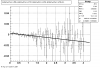
Victor's P diff (proximity)
|
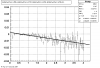
Victor's P diff (idtruth)
|
idtruth versus proximity
Victor's proximity plot
|
Victor's idtruth
|
bfcMixer.C Reshape
b>Date: Wednesday, 18 April 2007Time: 12:21:45
Topic: Embedding Reshape
18 April 2007 12:21:56
Talked to Yuri on Monday (16th)
He would like 3 things worked on.
1. Integration of MC generation part into bfcMixer.C
Basically all kumac commands can be done in macro using gstar.
These would become part of "chain one"
Also need to read in a tag or MuDst file to find vertex to use for generating particles.
Can probably see how this works from bfc.C itself as bfc.C(1) creates particles and runs them through reconstruction.
- actually I could not it is inside bfc.C or StBFChain because it is part of St_geant_Maker
2. Change Hit Mover so that it does not move hits derived from MC info (based on ID truth %age)
3. [I forgot what 3 was!]
Rough sketch of chain modifications for #1
Current bfcMixer
(StChain)Chain
(StBFChain)daqChain<--daq file
(StBFChain simChain<--fz file
<---.dat file with vertex positions
MixerMaker
(StBFChain)recoChain
New bfcMixer
(StChain)Chain
(
StBFChain)daqChain<--daq file
(StBFChain)simChain
|
Geant-?-SetGeantMaker<--tags file
MixerMaker
(StBFChain)recoChain
Break down into sub-tasks.
a) Run bfcMixer.C on a daq file with an associated fz and data file (to check that it works!)
b) Ignore fz file and generate MC particle (any!) on the fly
c) reading from tags file generate MC particles at desired vertex & with desired mult.
d) tidy up specify parameter interface (p distn, geant ID etc.)
Embedding Procedures
Overview
This document lists the procedures used for requesting embedding, running embedding jobs, and retrieving data. Please note that some steps require privileged accounts.
Embedding Documentation
Overview
The purpose of embedding is to provide physicists with a known; Monte Carlo tracks, where the kinematics and particle type is known exactly, are introduced into the realistic environment seen in the analysis - a real data event. How reconstruction preforms on these "standard candle" tracks provides a baseline which can be used to correct for acceptance and effciency effects in various analyses.
In STAR, embedding is achieved with a set of software tools - Monte Carlo simulation software, as well as the tools for real data event reconstruction - accessed through a suite of scripts. These documents attempt to provide an introduction to the scripts and their use, but the STAR collaborator is referred to the separate web pages maintained for Simulations and Reconstruction for deeper questions of the processes involved in those respective tasks.
Please note, the general procedure for embedding is:
- The Physics Working Group Convenor submits an embedding request. The request will be assigned a request number and priority by the Analysis Coordinator, see this page for more information.
- The Embedding Coordinator will coordinate the distribution of embedding requests. Users who wish to run their own embedding are encouraged to do so - but it must be verified with the Embedding Coordinator.
- The Embedding Coordinator is responsible for the QA of all embedding requests. When the Embedding Coordinator has verified that the test sample produced is acceptable, full production is authorized.
Obsolete documentations
Embedding Production Setup
This page describes how to set up embedding production. This procedure needs to be followed for any set of daq files/production version that requires embedding. Since this typically involves hacking the reconstruction chain, it is not advised that the typical STAR PA attempt this step. Please coordinate with a local embedding coordinator, and the overal Embedding coordinator (Olga).Note: The documentation here is very terse; it will be enriched as the documentation as a whole is iterated on. Patience is appreciated.
Get daq files from RCF.
| Grab a set of daq files from RCF which cover the lifetime of the run, the luminosity range experienced, and the conditions for the production. |
Rerun standard production but without corrections.
| bfc.C macros are located under ~starofl/bfc. Edit the submit.[Production] script to point to the daq files loaded (as above). |
Put tags files on disk.
| The results of the previous jobs will be .tags.root files located on HPSS. Retrieve the files, set a pointer for the tags files in the Production-specific directory under ~starofl/embedding. |
Now you're ready to start production.
Embedding Setup Off-site
Introduction
The purpose of this document is to describe step-by-step the setting up of embedding infrastructure on a remote site i.e. not at it's current home which is PDSF. It is based on the experience of setting up embedding at Birmingham's NP cluster (Bham). I will try to maintain a distinction between steps which are necessary in general and those which were specific to porting things to Bham. It should also be a useful guide for those wanting to run embedding at PDSF and needing to copy the relevant files into a suitable directory structure.Pre-requisites
Before trying to set up embedding on a remote site you should have:- a working local installation of the STAR library in which you are interested (or be satisified with your AFS-based library performance).
- a working mirror of the star database (or be satisfied with your connection to the BNL hosted db).
Collect scripts
The scripts are currently housed at PDSF in the 'starofl' account area. At the time of writing (and the time at which I set up embedding in Bham) they are not archived in CVS. The suggested way to collect them is to copy them into a directory in your own PDSF home account then tar and export it for installation on your local cluster. The top directory for embedding is /u/starofl/embedding . Under this directory there are several subdirectories of interest.- Those named after each production, e.g. P06ib which contain mixer macro and perl scripts
- Common which contains further subdirectories lists and csh and a submission perl script
- GSTAR which contains the kumac for running the simulation
mkdir embedding
cd embedding
mkdir Common
mkdir Common/lists
mkdir Common/csh
mkdir GSTAR
mkdir P06ib
mkdir P06ib/setup
Now it needs populating with the relevant files. In the following /u/user/embedding as an example of your new embedding directory in your user home directory.
cd /u/user/embedding
cp /u/starofl/embedding/getVerticesFromTags_v4.C .
cp -R /u/starofl/embedding/P06ib/EmbeddingLib_v4_noFTPC/ P06ib/
cp /u/starofl/embedding/P06ib/Embedding_sge_noFTPC.pl P06ib/
cp /u/starofl/embedding/P06ib/bfcMixer_v4_noFTPC.C P06ib/
cp /u/starofl/embedding/P06ib/submit.starofl.pl P06ib/submit.user.pl
cp /u/starofl/embedding/P06ib/setup/Piminus_101_spectra.setup P06ib/setup/
cp /u/starofl/embedding/GSTAR/phasespace_P06ib_revfullfield.kumac GSTAR/
cp /u/starofl/embedding/GSTAR/phasespace_P06ib_fullfield.kumac GSTAR/
cp /u/starofl/embedding/Common/submit_sge.pl Common/
You now have all the files need to run embedding. There are further links to make but as you are going to export them to your own cluster you need to make the links afterwards.
Alternatively you can run embedding on PDSF from your home directory. There are a number of change to make first though because the various perl scripts have some paths relating to the starofl account inside them.
For those planning to export to a remote site you should tar and/or scp the data. I would recommend tar so that you can have the original package preserved in case something goes wrong. E.g.
tar -cvf embedding.tar embedding/
scp embedding.tar remoteuser@mycluster.blah.blah:/home/remoteuser
Obviously this step is unnecessary if you intend to run from your PDSF account although you may still want to create a tar file so that you can undo any changes which are wrong.
Login to your remote cluster and extract the archive. E.gcd /home/remoteuser
tar -xvf embedding.tar
Script changes
The most obvious thing you will find are a number of places inside the perl scripts where the path or location for other scripts appears in the code. These must be changed accordingly.
P06ib/Embedding_sge_noFTPC.pl
changes to e.g.changes to e.g.changes to e.g.changes to e.g.
P06ib/EmbeddingLib_v4_noFTPC/Process_object.pm
changes to e.g.
changes to e.g.
This is because the location of tcsh was different and probably will be for you too.
Common/submit_sge.pl
changes to e.g.
Change relates to parsing the name of the directory with daq files in to extract the 'data vault' and 'magnetic field' which form part of job name and are used by Embedding_sge_noFTPC.pl (This may not make much sense right now and needs the detailed docs on each component. It is actually just a way to pass a file list with the same basename as the job). In the original script the path to the data is something like/dante3/starprod/daq/2005/cuProductionMinBias/FullField
whereas on Bham cluster it is/star/data1/daq/2005/cuProductionMinBias/FullField
and thus the pattern match in perl has to change in order to extract the same information. If you have a choice then choose your directory names with care!changes to e.g.
Change relates to the line printing the job submission shell script that this perl script writes and submits. The first line had to be changed such that it can correctly be identified as a sh script. I am not sure how original can ever have worked?changes to e.g.
This line prints part of the job submission script where the options for the job are specified. In SGE the job options can be in the file and not just on the command line. The extra options for Bham relate to our SGE setup. The-q
option provides the name of the queue to use, otherwise it uses the default which I did not want in this case. The other extra options are to make the environment and working diretory correct as they were not the default for us. This is very specific to each cluster. If your cluster does not have SGE then I imagine extensive changes to the part writing the job submission script would be necessary. The scripts use the ability of SGE to have job arrays of similar jobs so you would have to emulate that somehow.
- getVerticesFromTags_v4.C - none
- GSTAR/phasespace_P06ib_fullfield.kumac, GSTAR/phasespace_P06ib_fullfield.kumac - actually there are changes but they only relate to redefining particle decay modes for (anti-)Ξ and (anti-)Ω to go 100% to charged modes of interest. This is only relevant for strangeness group
- P06ib/bfcMixer_v4_noFTPC.C - checked carefully that
chain3->SetFlagsline actually sets the same flags since Andrew and I had to change the same flags e.g. add GeantOut option after I made orginal copy - P06ib/EmbeddingLib_v4_noFTPC/Chain_object.pm - none
- P06ib/EmbeddingLib_v4_noFTPC/EmbeddingUtilities.pm - there are lines where you may have to add the run numbers of the daq files which you are using so that they are recognised as either full field or reversed full field. In this example (Cu+Cu embedding in P06ib) the lines begin
and. This is also something that Andrew and I both changed after I made the original copy. - P06ib/submit.user.pl - changes here relate to setup that you want to run and not to the cluster or directory you are using i.e. which setup file to use, what daq directories to use and any pattern match on the file names (usually for testing purposes to avoid filling the cluster with useless jobs) although you probably want to change the
line! - P06ib/setup/Piminus_101_spectra.setup - any changes here relate to the simulation parameters of the job that you want to do and not to the cluster or directory you are using
Create links
A number of links are required. For example in the /u/starofl/embedding/P06ib there are the following links:daq_dir_2005_cuPMBFF -> /dante3/starprod/daq/2005/cuProductionMinBias/FullFielddaq_dir_2005_cuPMBRFF -> /dante3/starprod/daq/2005/cuProductionMinBias/ReversedFullFielddaq_dir_2005_cuPMBHTFF -> /eliza5/starprod/daq/2005/cucuProductionHT/FullField/daq_dir_2005_cuPMBHTRFF -> /eliza5/starprod/daq/2005/cucuProductionHT/ReversedFullFieldtags_dir_cuHT_2005 -> /eliza5/starprod/embedding/tags/P06ibdata -> /eliza12/starprod/embedding/datalists ->../Common/listscsh-> ../Common/cshLOG-> ../Common/LOG
tags_dir_cu_2005 -> /dante3/starprod/tags/P06ib/2005
That is it! Some things will probably need to be adapted to your circumstances but it should give you a good idea of what to do
Author: Lee Barnby, University of Birmingham (using starembed account)
Modified: A. Rose, Lawrence Berkeley National Laboratory (using starembed account)
Modified Birmingham Files
Upload of modified embedding infrastructure files used on Birmingham NP cluster for Cu+Cu for (anti-)Λ and K0S embedding request.Production Management
1) Usually embedding jobs are run in "HPSS" mode so the files end up in HPSS (via FTP). To transfer them from HPSS to disk copy the perl script ~starofl/hjort/getEmbed.pl and modify as needed. This script does at least two things that are not possible with, e.g., a command line hsi command: it only gets the files needed (usually the .geant and .event files) and it changes the permissions after the transfers. Note that if you do the transfers shortly after running the jobs the files will probably still be on the HPSS disk cache and transfers will be much fast than getting the files from tapes.2) To clean up old embedding files make your own copy of ~starofl/hjort/embedAge.pl and use as needed. Note that $accThresh determines the maximum access time in days of files that will not be deleted.
Running Embedding
This page describes how to run embedding jobs once the daq files and tags files are in place (see other page about embedding production setup).Basics:
Embedding code is located in production specific directories: ~starofl/embedding/P0xxx. The basic job submission template is typically called submit.starofl.pl in that directory.Jobs are usually run by user starofl but personal accounts with group starprod membership will work, too (but test first as the group starprod write permissions typically are not in place by default).
The script to submit a set of jobs is submit.[user].pl. The script should be modified to submit an embedding set from the the configuration file
~starofl/embedding/[Production]/setup/[Particle]_[set]_[ID].setup
where
[Particle] is the particle type submitted (Piminus for GEANTID=9, as set inside file)
[set] is the file set submitted (more on this later)
[ID] is the embedding request number
Test procedure:
The best way to test a particular job configuration is to run a single job in "DISK" mode (by selecting a specific daq file in your submission). In this mode all of the intermediate files, scripts, logs, etc., are saved on disk. The location will be under the "data" link in the working directory. You can then go and figure out which script failed, hack as necessary and and try to make things work...Details:
Notes
Overview
The document is intended as a forum for embedding group members to share information and notes.
LPP group (Dubna) activities
This page is intended to provide embedding progress for soft-photon study conducted by PPL (Dubna, JINR) group in Russia.- Requested embedding is based on request ID # 1103209240 and modified to:
- provide larger statistics for reco efficiency calculation
- extend acceptance parameters
- Related embedding jobs currently in production:
- ~420 kEvents done and loaded on the disk
- This is the embedding request and progress detals
- AuAu200, P05ic:
- Related embedding jobs to be planned:
- Jobs have not been started yet
- This is the embedding request and progress detals
- dAu200, P04if
AuAu200 photon embedding details
- Request details:
- Dataset and production: AuAu200, P05ic
- Embedded particles and multiplicity: 1000 Photons per event, total 500 kEvents
- zVertex = +-30
- Pt: 0.020 - 0.160 GeV
- eta: +-1.2
- full geant reconstruction
- Embedding Files on Disk at PDSF:
- Photon_201...215_spectra: /eliza5/starprod/embedding/P05ic/
- Photon_301...315_spectra: /eliza5/starprod/embedding/P05ic/
- Photon_401...415_spectra: /eliza7/starprod/embedding/P05ic/
- Photon_501...504_spectra: /eliza5/starprod/embedding/P05ic/
- Photon_505...515_spectra: /eliza7/starprod/embedding/P05ic/
- Photon_601...615_spectra: /eliza7/starprod/embedding/P05ic/
- Photon_701...715_spectra: /eliza12/starprod/embedding/P05ic/
- Photon_802...811,817,818_spectra: /eliza12/starprod/embedding/P05ic/
- Running Jobs status:
jobs QA and checking if this statistic is enough
dAu photon embedding details
- Request details:
- Dataset and production: dAu200, P04if
- Embedded particles and multiplicity: 1000 Photons per event, total 500 kEvents
- zVertex = +-50
- Pt: 0.020 - 0.160 GeV
- eta: +-1.2
- full geant reconstruction
- Running Jobs status:
have not been started yet
QA Status (OBSOLETE)
The full list of STAR embedding requests (Since August, 2010):http://drupal.star.bnl.gov/STAR/starsimrequest
The QA status of each request can be viewed in its history.
The information below are only valid for OLD embedding requests.
This document is intended to provide all the information available for each production, starting for the last or current production.
P06ib
QA Plots Phi(Feb 2009)
QA P06ib (Phi->K +K)
This is the QA for P06ib (Phi- > KK). reconstruction on Global Tracks (Kaons)
1. dEdx
Reconstruction on Kaon Daugthers. Plot shows MOntecarlo tracks and Ghost Tracsks.
/P06ib_dedx_Phi(Ghost).gif)
2. DCA Distributions
An original 3D histogram had been created and filled with pT, Eta and DCA as the 3 coordinates. Projection on PtBins and EtaBins had been made to create this "matrix" of plots. (MonteCarlo and MuDst) (MuDst taken from pdsf > /eliza12/starprod/reco/cuProductionMinBias/ReversedFullField/P06ib/2005/022/st_physics_adc_6022048_raw*.MuDst.root)
Pt Bin array used : { 0.5, 0.6, 0.8, 1.0} (moves down) and
Eta Bin array : {0.2, 0.5, 0.8, 1.0} (moves to the right)
For the Error bars, i used the option hist->Sumw2();
/dca_eta_pt_phi.gif)
3. NFit Distributions
Similarly An Original 3D Histogram had been created with Pt, Eta and Nfit as coordinates. Respective projections had been made in the same pT and Eta Bins as the DCa distributions. (MonteCarlo and MuDst)
Pt Bin array used : { 0.5, 0.6, 0.8, 1.0} (moves down) and
Eta Bin array : {0.2, 0.5, 0.8, 1.0} (moves to the right)
For the Error bars, i used the option hist->Sumw2();
/nfit_eta_pt_phi.gif)
4. Delta Vertex
The following are the Delta Vertex ( Vertex Reconstructed - Vertex Embedded) plot for the 3 diiferent coordinates (x, y and z) (Cuts of vz =30 cm , NFitCut= 25 are applied)
/Delta_vertex_Phi.gif)
5. Z Vertex and X vs Y vertex
/vertex_Phi.gif)
6. Global Variables : Phi and Rapidity
/y_f_phi(1).gif)
/phi_f_phi.gif)
7. Pt
Embedded Phi meson with flat pt (black)and Reconstructed Kaon Daugther (red).
/pt_f_phi.gif)
8. Randomness Plots
The following plots, are to check the randomness of the input Monte Carlo (MC) tracks.
/mc_pt_y_Phi_K.gif)
/mc_y_phi_phi_K.gif)
QA plots Rho (February 16 2009)
QA P06ib (Rho->pi+pi)
This is the QA for P06ib (Rho- > pi+pi). reconstruction on Global Tracks (pions)
1. dEdx
Reconstruction on Pion Daugthers.
2. DCA Distributions
An original 3D histogram had been created and filled with pT, Eta and DCA as the 3 coordinates. Projection on PtBins and EtaBins had been made to create this "matrix" of plots.
Pt Bin array used : { 0.5, 0.6, 0.8, 1.0} (moves down) and
Eta Bin array : {0.2, 0.5, 0.8, 1.0} (moves to the right)
For the Error bars, i used the option hist->Sumw2();
2b. Compared with MuDst
.gif)
3. NFit Distributions
Similarly An Original 3D Histogram had been created with Pt, Eta and Nfit as coordinates. Respective projections had been made in the same pT and Eta Bins as the DCa distributions.
Pt Bin array used : { 0.5, 0.6, 0.8, 1.0} (moves down) and
Eta Bin array : {0.2, 0.5, 0.8, 1.0} (moves to the right)
For the Error bars, i used the option hist->Sumw2();
3b. Reconstructed compared with MuDsts
.gif)
4. Delta Vertex
The following are the Delta Vertex ( Vertex Reconstructed - Vertex Embedded) plot for the 3 diiferent coordinates (x, y and z) (Cuts of vz =30 cm , NFitCut= 25 are applied)
5. Z Vertex and X vs Y vertex
6. Global Variables : Phi and Rapidity
7. Pt
Embedded Rho meson with flat pt (black)and Recosntructed Pion (red).
8. Randomness Plots
The following plots, are to check the randomness of the input Monte Carlo (MC) tracks.
.gif)
QA plots Rho (October 21 2008)
Some QA plots for Rho:
MiniDst files are at PDSF under the path /eliza13/starprod/embedding/p06ib/MiniDst/rho_101/*.minimc.root
MuDst files are at PDSF under /eliza13/starprod/embedding/P06ib/MuDst/10*/*.MuDst.root Reconstruction had been done on PionPlus.
DCA and Nfit Distributions had been scaled by the Integral in different pt ranges
QAPlots_D0
Some QA Plots for D0 located under the path :
/eliza12/starprod/embedding/P06ib/D0_001_1216876386/*
/eliza12/starprod/embedding/P06ib/D0_002_1216876386/ -> Directory empty
Global pairs are used as reconstructed tracks. SOme quality tractst plotiing level were :
Vz Cut 30 cm ;
NfitCut : 25,
Ncommonhits : 10 ;
maxDca :1 cm ; Assuming D0- >pi + pi
P05id
P05id Cu+Cu Embedding
Hit level check-up : At the Hit level the results look in good agreement.
- Missing/Dead Areas (PiMinus): The next graphs show dead sectors for embeded data and real data as well.
- Missing/Dead Areas (PiPlus)
- Track Residuals PiMinus
- Track Residuals PiPlus
- dEdx Comparisons
 | |
 | |
 | |
 | |
 | |
 |
 | |
 | |
 | |
 | |
 | |
 |
The following are results of dEdx calibration from embedding for Pi Minus. Graphs 1 and 2 are Dedx vs Momentum grapsh where Green dots are the MonteCarlo Tracks reconstructed from Embedding and Black dots are Data. In Graph Number 2, dots are Data and solid lines show Bichsel parametrisation with a factor of 1/2 offset. In the Last Graph a projection on dEdx axis is done and a MIP of 1.26 and 1.18 are shown.
 | |
 |
P08ic -Jpsi(Test)
QA P08ic J/Psi -> ee+
This is the QA for P08id (jPsi - > ee). Reconstructin on Global Tracks and just Electrons (Positrons).
1. dEdx
2. DCA Distributions
An original 3D histogram had been created and filled with pT, Eta and DCA as the 3 coordinates. Projection on PtBins and EtaBins had been made to create this "matrix" of plots.
Pt Bin array used : { 0.5, 0.6, 0.8, 1.0} (moves down) and
Eta Bin array : {0.2, 0.5, 0.8, 1.0} (moves to the right)
For the Error bars, i used the option hist->Sumw2();
3. NFit Distributions
Similarly An Original 3D Histogram had been created with Pt, Eta and Nfit as coordinates. Respective projections had been made in the same pT and Eta Bins as the DCa distributions.
Pt Bin array used : { 0.5, 0.6, 0.8, 1.0} (moves down) and
Eta Bin array : {0.2, 0.5, 0.8, 1.0} (moves to the right)
For the Error bars, i used the option hist->Sumw2();
4. Delta Vertex
The following are the Delta Vertex ( Vertex Reconstructed - Vertex Embedded) plot for the 3 diiferent coordinates (x, y and z)
5. Z Vertex and X vs Y vertex
6. Global Variables : Phi and Rapidity
7. Pt
Embedded J/Psi with flat pt (black)and Recosntructed Electrons (red).

8. Randomness Plots
The following plots, are to check the randomness of the input Monte Carlo (MC) tracks.
P08id (AXi -> RecoPiPlus)
AXi-> Lamba + Pion + ->P + Pion - + Pion +
(03 08 2009)
1. Dedx
2.Dca
An original 3D histogram had been created and filled with pT, Eta and DCA as the 3 coordinates. Projection on PtBins and EtaBins had been made to create this "matrix" of plots.
Pt Bin array used : { 0.5, 0.6, 0.8, 1.0} (moves down) and
Eta Bin array : {0.2, 0.5, 0.8, 1.0} (moves to the right)
For the Error bars, i used the option hist->Sumw2();
3. Nfit
Similarly An Original 3D Histogram had been created with Pt, Eta and Nfit as coordinates. Respective projections had been made in the same pT and Eta Bins as the DCa distributions.
Pt Bin array used : { 0.5, 0.6, 0.8, 1.0} (moves down) and
Eta Bin array : {0.2, 0.5, 0.8, 1.0} (moves to the right)
For the Error bars, i used the option hist->Sumw2();

4. Delta Vertex
5. Z Vertex and X vs Y vertex
6. Global Variables : Phi and Rapidity
7. pt

8. Randomness

P08id (Omega -> RecoPiMinus)
Omega-> Lamba + K - -> P + Pion - + K -
(03 08 2009)
1. Dedx
Reconstruction on pion Minus and Proton Daugthers. 2 different plots are shown just for the sake of completenees.... Reconsructing on Kaon had very few statistics
| Reco PionMinus | Reco Proton |
 |  |
2.Dca
An original 3D histogram had been created and filled with pT, Eta and DCA as the 3 coordinates. Projection on PtBins and EtaBins had been made to create this "matrix" of plots.
Pt Bin array used : { 0.5, 0.6, 0.8, 1.0} (moves down) and
Eta Bin array : {0.2, 0.5, 0.8, 1.0} (moves to the right)
For the Error bars, i used the option hist->Sumw2();
*.Reconstructing on Pion
*. Reconstructing on Proton
3. Nfit
Similarly An Original 3D Histogram had been created with Pt, Eta and Nfit as coordinates. Respective projections had been made in the same pT and Eta Bins as the DCa distributions.
Pt Bin array used : { 0.5, 0.6, 0.8, 1.0} (moves down) and
Eta Bin array : {0.2, 0.5, 0.8, 1.0} (moves to the right)
For the Error bars, i used the option hist->Sumw2();
*. Reconstructing Pion
*. Reconstructing Proton
4. Delta Vertex
When reconstructed in Pion Minus and Proton it turns out to have the same ditreibutions so I just posted one of them
5. Z Vertex and X vs Y vertex
6. Global Variables : Phi and Rapidity
| Reco Pion | Reco Kaon |
 |  |
 |  |
7. pt
8. Randomness


P08id (phi ->KK) (March 05 2009)
QA Phi->KK (March 05 2009)
1. Dedx
Reconstruction on Kaon Daugthers. 2 different plots are shown just for the sake of completenees....
/Dedx_P08id_Phi_030509(Ghost.gif)
/Dedx_P08id_Phi_030509.gif)
2.Dca
An original 3D histogram had been created and filled with pT, Eta and DCA as the 3 coordinates. Projection on PtBins and EtaBins had been made to create this "matrix" of plots.
Pt Bin array used : { 0.5, 0.6, 0.8, 1.0} (moves down) and
Eta Bin array : {0.2, 0.5, 0.8, 1.0} (moves to the right)
For the Error bars, i used the option hist->Sumw2();
/DCA_eta_pt_P08id_Phi_030509.gif)
3. Nfit
Similarly An Original 3D Histogram had been created with Pt, Eta and Nfit as coordinates. Respective projections had been made in the same pT and Eta Bins as the DCa distributions.
Pt Bin array used : { 0.5, 0.6, 0.8, 1.0} (moves down) and
Eta Bin array : {0.2, 0.5, 0.8, 1.0} (moves to the right)
For the Error bars, i used the option hist->Sumw2();
/Nfit_eta_pt_P08id_Phi_030509.gif)
4. Delta Vertex
/DeltaVertex_P08id_Phi_030509.gif)
5. Z Vertex and X vs Y vertex
/Vertex_P08id_Phi_030509.gif)
6. Global Variables : Phi and Rapidity
/Phi_P08id_Phi_030509.gif)
/Rapidity_P08id_Phi_030509.gif)
7. pt
/pT_P08id_Phi_030509.gif)
8. Randomness
/Y_pT_P08id_Phi_030509.gif)
/pT_Phi_P08id_Phi_030509.gif)
P08id (phi ->KK)
QA P08id (Phi->KK)
This is the QA for P08id (phi - > KK). econstructin on Global Tracks and just Kaons. Macro from Xianglei used (I found the QA macro very familiar). scale factor of 1.38 applied.
1. dEdx
Reconstruction on Kaon Daugthers. 2 different plots are shown just to see how Montecarlo looks on top of the Ghost Tracks
/dedx_f1_38(1).gif)
/dedx_v2_f1_38.gif)
2. DCA Distributions
An original 3D histogram had been created and filled with pT, Eta and DCA as the 3 coordinates. Projection on PtBins and EtaBins had been made to create this "matrix" of plots.
Pt Bin array used : { 0.5, 0.6, 0.8, 1.0} (moves down) and
Eta Bin array : {0.2, 0.5, 0.8, 1.0} (moves to the right)
For the Error bars, i used the option hist->Sumw2();
/dca_eta_pt(1).gif)
3. NFit Distributions
Similarly An Original 3D Histogram had been created with Pt, Eta and Nfit as coordinates. Respective projections had been made in the same pT and Eta Bins as the DCa distributions.
Pt Bin array used : { 0.5, 0.6, 0.8, 1.0} (moves down) and
Eta Bin array : {0.2, 0.5, 0.8, 1.0} (moves to the right)
For the Error bars, i used the option hist->Sumw2();
/nfit_eta_pt(1).gif)
4. Delta Vertex
The following are the Delta Vertex ( Vertex Reconstructed - Vertex Embedded) plot for the 3 diiferent coordinates (x, y and z)
/DeltaVX.gif)
/DeltaVY.gif)
/DeltaVZ.gif)
5. Z Vertex and X vs Y vertex
/vertex_1_38.gif)
6. Global Variables : Phi and Rapidity
/phi_f1_38.gif)
/y_f1_38.gif)
7. Pt
Embedded Phi meson with flat pt (black)and Recosntructed Kaons (red).
/pt_f1_38.gif)
8. Randomness Plots
The following plots, are to check the randomness of the input Monte Carlo (MC) tracks.
/mc_pt_phi.gif)
/mc_pt_y.gif)
P08id(ALambda -> P, Pion)
QA ALambda->P, pi (03 08 2009)
1. Dedx
Reconstruction on Proton and Pion Daugthers. 2 different plots are shown just for the sake of completenees....
| Reco Proton | Reco Pion |
 |  |
2.Dca
An original 3D histogram had been created and filled with pT, Eta and DCA as the 3 coordinates. Projection on PtBins and EtaBins had been made to create this "matrix" of plots.
Pt Bin array used : { 0.5, 0.6, 0.8, 1.0} (moves down) and
Eta Bin array : {0.2, 0.5, 0.8, 1.0} (moves to the right)
For the Error bars, i used the option hist->Sumw2();
*.Reconstructing on Proton
*. Reconstructing on Pion
3. Nfit
Similarly An Original 3D Histogram had been created with Pt, Eta and Nfit as coordinates. Respective projections had been made in the same pT and Eta Bins as the DCa distributions.
Pt Bin array used : { 0.5, 0.6, 0.8, 1.0} (moves down) and
Eta Bin array : {0.2, 0.5, 0.8, 1.0} (moves to the right)
For the Error bars, i used the option hist->Sumw2();
*. Reconstructing Proton
*. Reconstructing Pion
4. Delta Vertex
When reconstructed in Proton and pions it turns out to have the same ditreibutions so I just posted one of them
5. Z Vertex and X vs Y vertex
6. Global Variables : Phi and Rapidity
| Reco Proton | Reco Pion |
 |  |
 |  |
7. pt
8. Randomness
P08id(Xi -> Reco(PiMinus)
Xi-> Lamba + Pion - ->P + Pion - + Pion -
(03 08 2009)
1. Dedx
Reconstruction on PI Minus
2.Dca
An original 3D histogram had been created and filled with pT, Eta and DCA as the 3 coordinates. Projection on PtBins and EtaBins had been made to create this "matrix" of plots.
Pt Bin array used : { 0.5, 0.6, 0.8, 1.0} (moves down) and
Eta Bin array : {0.2, 0.5, 0.8, 1.0} (moves to the right)
For the Error bars, i used the option hist->Sumw2();
3. Nfit
Similarly An Original 3D Histogram had been created with Pt, Eta and Nfit as coordinates. Respective projections had been made in the same pT and Eta Bins as the DCa distributions.
Pt Bin array used : { 0.5, 0.6, 0.8, 1.0} (moves down) and
Eta Bin array : {0.2, 0.5, 0.8, 1.0} (moves to the right)
For the Error bars, i used the option hist->Sumw2();
4. Delta Vertex
5. Z Vertex and X vs Y vertex
6. Global Variables : Phi and Rapidity
7. pt
8. Randomness
Phi->KK(Mar 12)
Please find the QA plots here
The data looks good.
Reconstructed phi meson has small rapidity dependence.
Yuri_Test_PionMinus_032009
 QA PionMinus
P04if
-
Hit level check-up:
Previous results - May 2002
This document is intended to provide all the information available for previous productions such that results for Quality Control studies and Productions Cross checks. Part of quality control studies include identification of missing/dead detector areas, distance of closest approach distributions (dca), and fit points distributions(Nfit). As part of production cross checks, some results in centrality dependance and efficiency are shown
Quality Control
These are dedx vs P graphs. All of them show reasonable agreement with data.(Done on May 2002)
| Pi Minus | K Minus | Proton |
| Pi Plus | K Plus | P Bar |

PI PLUS. In the following dca distributions some discrepancy is shown. Due to secondaries?
| Peripheral 0.1 GeV/c < pT < 0.2 Gev/c | MinBias 0.2 GeV/c < pT < 0.3 Gev/c | Central 0.3 GeV/c <pT < 0.4 GeV/c |
PI MINUS. Some discrepancy is shown. Due to secondaries?
| Peripheral 0.1 GeV/c < pT < 0.2 Gev/c | MinBias 0.2 GeV/c < pT < 0.3 Gev/c | Central 0.3 GeV/c <pT < 0.4 GeV/c |

K PLUS. In the following dca distributions Good agreement with data is shown.
| Peripheral 0.1 GeV/c < pT < 0.2 Gev/c | MinBias 0.2 GeV/c < pT < 0.3 Gev/c | Central 0.3 GeV/c <pT < 0.4 GeV/c |
K MINUS. In the following dca distributions Good agreement with data is shown.
| Peripheral 0.1 GeV/c < pT < 0.2 Gev/c | MinBias 0.2 GeV/c < pT < 0.3 Gev/c | Central 0.3 GeV/c <pT < 0.4 GeV/c |
PROTON. The real data Dca distribution is wider, especially at low pT -> Most likely due to secondary tracks in the sample. A tail from background protons dominating distribution at low pt can be clearly seen. Expected deviation from the primary MC tracks.
| Peripheral 0.2 GeV/c < pT < 0.3 Gev/c | MinBias 0.5 GeV/c < pT < 0.6 Gev/c | Central 0.7 GeV/c <pT < 0.8 GeV/c |
Pbar. The real data Dca distribution is wider, especially at low pT -> Most likely due to secondary tracks in the sample.
| Peripheral 0.2 GeV/c < pT < 0.3 Gev/c | MinBias 0.3 eV/c < pT < 0.4 Gev/c | Central 0.5 GeV/c <pT < 0.6 GeV/c |
PI PLUS. Good agreement with data is shown.
| Peripheral 0.1 GeV/c < pT < 0.2 Gev/c | MinBias 0.2 GeV/c < pT < 0.3 Gev/c | Central 0.3 GeV/c <pT < 0.4 GeV/c |
PI MINUS. Good agreement with data is shown.
| Peripheral 0.1 GeV/c < pT < 0.2 Gev/c | Peripheral 0.2 GeV/c < pT < 0.3 Gev/c | Peripheral 0.3 GeV/c < pT < 0.4 Gev/c |

K PLUS. Good agreement with data is shown.
| Peripheral 0.1 GeV/c < pT < 0.2 Gev/c | MinBias 0.2 GeV/c < pT < 0.3 Gev/c | Central 0.3 GeV/c <pT < 0.4 GeV/c |
K MINUS. Good agreement with data is shown.
| Peripheral 0.1 GeV/c < pT < 0.2 Gev/c | Peripheral 0.2 GeV/c < pT < 0.3 Gev/c | Peripheral 0.3 GeV/c < pT < 0.4 Gev/c |
PROTON. Good agreement with data is shown.
| Peripheral 0.2 GeV/c < pT < 0.3 Gev/c | Peripheral 0.3 GeV/c < pT < 0.4 Gev/c | Peripheral 0.5 GeV/c < pT < 0.6 Gev/c |
Pbar. Good agreement with data is shown.
| Peripheral 0.2 GeV/c < pT < 0.3 Gev/c | Peripheral 0.3 GeV/c < pT < 0.4 Gev/c | Peripheral 0.5 GeV/c < pT < 0.6 Gev/c |
Reconstruction
Field Issues
This is meant to be a central location for finding reconstruction-related items which have some field dependences.
- AuAu200 (2005)
-
proton-Lambda HBT
- h+/h- ratio (odd pt shape, but same between fields)
- Track and V0 reconstruction (general agreement between fields?)
- h+/h- ratio (odd pt shape, but same between fields)
- AuAu200 (2003)
- Xi decay analyses - use of a greater decay length cut seemed to alleviate the differences seen in Xi+/Xi- ratio
Reconstruction Code QA
Cross reference to Reconstruction Code QA
STAR Reconstruction Software
| STAR Computing | |
| STAR Reconstruction Software | |
| Hypernews forums: Tracking/Fitting Event Vertex/Primaries Subscribe | Y. Fisyak, S. Margetis, C. Pruneau |
SVT Alignment and June 2006 review
Summary pages
SVT+SSD Alignment, Run VII (2007)
Alignment
Software for Tracking Upgrade (Challenge week 01/17/06-01/24/06)
Agenda Result of Kolmogorov's tests for QA histograms for different versions of STAR codes
New STAR magnetic field
When and what dEdx Prediction for P10 has to be used
Reconstruction plans
Usage of Truth information in reconstruction.
STAR track flags.
ITTF
integration week January 2004 p-p software workshop at BNL 2001/11/19
Final Agenda and Talks . Minutes from the meeting are here. Integrated Tracking Task Force (ITTF)
The official web cite maintained by Claude Pruneau is here .
See also the STAR Kalman filter documentation created by Claude Pruneau. LBL Tracking review report
Available in MS-WORD and PDF format. Some talks given are linked here. Kalman in BABAR
A note on Kalman is here in .ps format. Kalman in ATLAS
Igor Gavrilenko's presentation for 5/22/00 in power point format, ATLAS internal note with xKalman description.
Spiros talk on video meeting about it on June/2/2000 is here in power point format. Flagging scheme for tracks failing Kalman fitter (Al Saulys) Kalman Fitter Evaluation page-I (Al Saulys) Kalman Fitter Evaluation page-II (Lee Barnby) Kalman Fitter for V0 search (Al Saulys) Kalman in STAR
A preliminary writeup of the Kalman implementation in STAR in use during 2001. Current Work on Tracking/Fitting Tools
The group is currently looking into some of the options for improving the global tracking and fitting. These options include an implementation of GEANE as a universal track propagation engine, providing an interface between tracking and geometry/material info, and using Kalman filtering techniques to obtain the best estimation of track parameters. Kalman Tracking/Fitting Tools
Kalman literature (Spiros Margetis)
Simulation
Welcome to the Simulation Pages!
Please note that most of the material posted before October 2006 is located at the older web site which we'll keep for reference, for the time being. See sections below for most recent additions and information.
For making a new simulation production request, please consult the STAR Simulations Requests interface.
Adding a New Detector to STAR
The STAR Geometry Model
![]()
Geometry Definition
Users wishing to develop and integrate new detector models into the STAR framework will be intersted in the following links:
- The STAR AgML reference guide.
- The STAR AgML example shapes.
- List of Default AgML Materials
- The AgML Tutorials is a good place to get started with AgML development.
- An annotated example, the AgML Example: The Beam Beam Counters, is also available.
- Another example, the FGT geometry
Tracking Interface (Stv)
Exporting detector hits
- Implement a hit class based on StEvent/StHit
- Implement a hit collection
- Implement an iterator over your hit collection based on StEventUtilities/StHitIter
- Add your hit iterator to the StEventUtitlies/StEventHitIter
Implementing a custom seed finder
ID Truth
ID truth is an ID which enables us to determine which simulated particle was principally responsible for the creation of a hit in a detector, and eventually the physics objects (clusters, points, tracks) which are formed from them. The StHit class has a member function which takes two arguements:
- idTru -- the primary key of the simulated particle, i.e. "track_p" in the g2t hit structure
- qaTru -- the quality of the truth value, defined as the dominant contributor to the hit, cluster, point or track.
When hits are built up into clusters, the clustering algorithm should set the idtruth value for the cluster based on the dominant contributor of the hits which make up the cluster.
When clusters are associated into space points, the point finding algorithm should set the idtruth value for the point. In the event that two clusters are combined with two different idTruth values, you should set idTruth = 0.
Interface to Starsim
The interface between starsim and reconstruction is briefly outlined here
- You do not have access to view this node
Information about geometries used in production and which geometries to use in simulations may be found in the following links:
- Existing Geometry Tags used in Production
- The STAR Geometry in simulation & reconstruction contains useful information on the detector configurations associated with a unique geometry tag. Production geometry tags state the year for which the tag is valid, and a letter indicating the revision level of the geometry. For example, "y2009c" indicates the third revision of the 2009 configuration of the STAR detector. Users wishing to run starsim in their private areas are encouraged to use the most recent revision for the year in which they want to compare to data.
Comparisons between the original AgSTAR model and the new AgML model of the detector may be found here:
- Comparisons between AgML vs AgSTAR Comparison demonstrate the level of equivalence between AgML and the original AgSTAR geometries.
- Comparisons between You do not have access to view this node HITS, for simple simulations run in starsim.
- Comparisons between AgML vs AgSTAR tracking comparison
AgML Project Overview and Readiness for 2012
HOWTO Use Geometries defined in AgML in STARSIM
AgML geometries are available for use in simulation using the "eval" libraries.
$ starver eval
The geometries themselves are available in a special library, which is setup for backwards compatability with starsim. To use the geometries you load the "xgeometry.so" library in a starsim session, either interactively or in a macro:
starsim> detp geom y2012
starsim> gexe $STAR_LIB/xgeometry.so
starsim> gclos all
HOWTO Use Geometries defined in AgML in the Big Full Chain
AgML geometries may also be used in reconstruction. To access them, the "agml" flag should be provided in the chain being run:
e.g
root [0] .L bfc.C
root [1] bfc(nevents,"y2012 agml ...", inputFile);
Geometry in Preparation: y2012Major changes: 1. Support cone, ftpc, ssd, pmd removed.
2. Inner Detector Support Module (IDSM) added
3. Forward GEM Tracker (FGTD) added
Use of AgML geometries within starsim:
$ starver eval
$ starsim
starsim> detp geom y2012
starsim> gexe $STAR_LIB/xgeometry.so
starsim> gclos all
Use of AgML geometries within the big full chain:
$ root4star
root [0] .L bfc.C
root [1] bfc(0,"y2012 agml ...",inputFile);
|
Current (10/24/2011) configuration of the IDSM with FGT inside --  |
 |
AgML Example: The Beam Beam Counters
-
<Document file="StarVMC/Geometry/BbcmGeo/BbcmGeo.xml">
-
<!--
-
Every AgML document begins with a Document tag, which takes a single "file"
-
attribute as its arguement.
-
-
-->
-
-
-
<Module name="BbcmGeo" comment=" is the Beam Beam Counter Modules GEOmetry " >
-
<!--
-
The Module tag declares an AgML module. The name should consist of a four
-
letter acronym, followed by the word "geo" and possibly a version number.
-
-
e.g. BbcmGeo, EcalGeo6, TpceGeo3a, etc...
-
-
A mandatory comment attribute provides a short description of which detector
-
is implemented by the module.
-
-
-->
-
-
<Created date="15 march 2002" />
-
<Author name="Yiqun Wang" />
-
<!-- The Created and Author tags accept a free-form date and author, for the
-
purposes of documentation. -->
-
-
-
<CDE>AGECOM,GCONST,GCUNIT</CDE>
-
<!-- The CDE tag provides some backwards compatability features with starsim.
-
AGECOM,GCCONST and GCUNIT are fine for most modules. -->
-
-
<Content>BBCM,BBCA,THXM,SHXT,BPOL,CLAD</Content>
-
<!-- The Content tag should declare the names of all volumes which are
-
declared in the detector module. A comma-separated list. -->
-
-
<Structure name="BBCG" >
-
<var name="version" />
-
<var name="onoff(3)" />
-
<var name="zdis(2)" />
-
</Structure>
-
<!-- The structure tag declares an AgML structure. It is similar to a c-
-
struct, but has some important differences which will be illustrated
-
later. The members of a Structure are declared using the var tag. By
-
default, the type of a var will be a float.
-
-
Arrays are declared by enclosing the dimensions of the array in
-
parentheses. Only 1D and 2D arrayes are supported. e.g.
-
-
<var name="x(3)" /> allowed
-
<var name="y(3,3)" /> allowed
-
<var name="z(4,4,4)" /> not allowed
-
-
Types may be declared explicitly using the type parameter as below.
-
Valid types are int, float and char. char variables should be limited
-
to four-character strings for backwards compatability with starsim.
-
Arrays of chars are allowed, in which case you may treat the variable
-
as a string of length Nx4, where N is the dimension of the array.
-
-
-->
-
-
<Structure name="HEXG">
-
<var name="type" type="float" />
-
<var name="irad" type="float" />
-
<var name="clad" type="float" />
-
<var name="thick" type="float" />
-
<var name="zoffset" type="float" />
-
<var name="xoffset" type="float" />
-
<var name="yoffset" type="float" />
-
</Structure>
-
-
<varlist type="float">
-
actr,srad,lrad,ztotal,x0,y0,theta0,phi0,xtrip,ytrip,rtrip,thetrip,rsing,thesing
-
</varlist>
-
<!-- The varlist tag allows you to declare a list of variables of a stated type.
-
The variables will be in scope for all volumes declared in the module.
-
-
Variables may be initialized using the syntax
-
var1/value1/ , var2/value2/, var3, var4/value4/ ...
-
-
Arrays of 1 or 2 dimensions may also be declared. The Assign tag may
-
be used to assign values to the arrays:
-
-
<Assign var="ARRAY" value="{1,2,3,4}" />
-
-->
-
-
<varlist type="int">I_trip/0/,J_sing/0/</varlist>
-
-
<Fill name="BBCG" comment="BBC geometry">
-
<var name="Version" value="1.0" comment=" Geometry version " />
-
<var name="Onoff" value="{3,3,3}" comment=" 0 off, 1 west on, 2 east on, 3 both on: for BBC,Small tiles,Large tiles " />
-
<var name="zdis" value="{374.24,-374.24}" comment=" z-coord from center in STAR (715/2+6*2.54+1=373.8) " />
-
</Fill>
-
<!-- The members of a structure are filled inside of a Fill block. The Fill
-
tag specifies the name of the structure being filled, and accepts a
-
mandatory comment for documentation purposes.
-
-
The var tag is used to fill the members of the structure. In this
-
context, it accepts three arguements: The name of the structure member,
-
the value which should be filled, and a mandatory comment for
-
documentation purposes.
-
-
The names of variables, structures and structure members are case-
-
insensitive.
-
-
1D Arrays are filled using a comma separated list of values contained in
-
curly brackets...
-
-
e.g. value="{1,2,3,4,5}"
-
-
2D Arrays are filled using a comma and semi-colon separated list of values
-
-
e.g. value="{11,12,13,14,15; This fills an array dimensioned
-
21,22,23,24,25; as A(3,5)
-
31,32,33,34,35;}"
-
-
-->
-
-
-
<Fill name="HEXG" comment="hexagon tile geometry" >
-
<var name="Type" value="1" comment="1 for small hex tile, 2 for large tile " />
-
<var name="irad" value="4.174" comment="inscribing circle radius =9.64/2*sin(60)=4.174 " />
-
<var name="clad" value="0.1" comment="cladding thickness " />
-
<var name="thick" value="1.0" comment="thickness of tile " />
-
<var name="zoffset" value="1.5" comment="z-offset from center of BBCW (1), or BBCE (2) " />
-
<var name="xoffset" value="0.0" comment="x-offset center from beam for BBCW (1), or BBCE (2) " />
-
<var name="yoffset" value="0.0" comment="y-offset center from beam for BBCW (1), or BBCE (2) " />
-
</Fill>
-
-
<Fill name="HEXG" comment="hexagon tile geometry" >
-
<var name="Type" value="2" comment="1 for small hex tile, 2 for large tile " />
-
<var name="irad" value="16.697" comment="inscribing circle radius (4x that of small one) " />
-
<var name="clad" value="0.1" comment="cladding of tile " />
-
<var name="thick" value="1.0" comment="thickness of tile " />
-
<var name="zoffset" value="-1.5" comment="z-offset from center of BBCW (1), or BBCE (2) " />
-
<var name="xoffset" value="0.0" comment="x-offset center from beam for BBCW (1), or BBCE (2) " />
-
<var name="yoffset" value="0.0" comment="y-offset center from beam for BBCW (1), or BBCE (2) " />
-
</Fill>
-
-
<Use struct="BBCG"/>
-
<!-- An important difference between AgML structures and c-structs is that
-
only one instance of an AgML structure is allowed in a geometry module,
-
and there is no need for the user to create it... it is automatically
-
generated. The Fill blocks store multiple versions of this structure
-
in an external name space. In order to access the different versions
-
of a structure, the Use tag is invoked.
-
-
Use takes one mandatory attribute: the name of the structure to use.
-
By default, the first set of values declared in the Fill block will
-
be loaded, as above.
-
-
The Use tag may also be used to select the version of the structure
-
which is loaded.
-
-
Example:
-
<Use struct="hexg" select="type" value="2" />
-
-
The above example loads the second version of the HEXG structure
-
declared above.
-
-
NOTE: The behavior of a structure is not well defined before the
-
Use operator is applied.
-
-
-->
-
-
-
<Print level="1" fmt="'BBCMGEO version ', F4.2" >
-
bbcg_version
-
</Print>
-
<!-- The Print statement takes a print "level" and a format descriptor "fmt". The
-
format descriptor follows the Fortran formatting convention
-
-
(n.b. Print statements have not been implemented in ROOT export
-
as they utilize fortran format descriptors)
-
-->
-
-
-
<!-- small kludge x10000 because ROOT will cast these to (int) before computing properties -->
-
<Mixture name="ALKAP" dens="1.432" >
-
<Component name="C5" a="12" z="6" w="5 *10000" />
-
<Component name="H4" a="1" z="1" w="4 *10000" />
-
<Component name="O2" a="16" z="8" w="2 *10000" />
-
<Component name="Al" a="27" z="13" w="0.2302 *10000" />
-
</Mixture>
-
<!-- Mixtures and Materials may be declared within the module... this one is not
-
a good example, as there is a workaround being used to avoid some issues
-
with ROOT vs GEANT compatability. -->
-
-
-
<Use struct="HEXG" select="type" value="1 " />
-
srad = hexg_irad*6.0;
-
ztotal = hexg_thick+2*abs(hexg_zoffset);
-
-
<Use struct="HEXG" select="type" value="2 " />
-
lrad = hexg_irad*6.0;
-
ztotal = ztotal+hexg_thick+2*abs(hexg_zoffset); <!-- hexg_zoffset is negative for Large (type=2) -->
-
-
<!-- AgML has limited support for expressions, in the sense that anyhing which
-
is not an XML tag is passed (with minimal parsing) directly to the c++
-
or mortran compiler. A few things are notable in the above lines.
-
-
(1) Lines may be optionally terminated by a ";", but...
-
(2) There is no mechanism to break long lines across multiple lines.
-
(3) The members of a structure are accessed using an "_", i.e.
-
-
hexg_irad above refers to the IRAD member of the HEXG structure
-
loaded by the Use tag.
-
-
(4) Several intrinsic functions are available: abs, cos, sin, etc...
-
-->
-
-
<Create block="BBCM" />
-
<!-- The Create operator creates the volume specified in the "block"
-
parameter. When the Create operator is invoked, execution branches
-
to the block of code for the specified volume. In this case, the
-
Volume named BBCM below. -->
-
-
<If expr="bbcg_OnOff(1)==1|bbcg_OnOff(1)==3">
-
-
<Placement block="BBCM" in="CAVE"
-
x="0"
-
y="0"
-
z="bbcg_zdis(1)"/>
-
<!-- After the volume has been Created, it is positioned within another
-
volume in the STAR detector. The mother volume may be specified
-
explicitly with the "in" attribute.
-
-
The position of the volume is specified using x, y and z attributes.
-
-
An additional attribute, konly, is used to indicate whether or
-
not the volume is expected to overlap another volume at the same
-
level in the geometry tree. konly="ONLY" indicates no overlap and
-
is the default value. konly="MANY" indicates overlap is possible.
-
-
For more info on ONLY vs MANY, consult the geant 3 manual.
-
-->
-
-
</If>
-
-
<If expr="bbcg_OnOff(1)==2|bbcg_OnOff(1)==3" >
-
<Placement block="BBCM" in="CAVE"
-
x="0"
-
y="0"
-
z="bbcg_zdis(2)">
-
<Rotation alphay="180" />
-
</Placement>
-
<!-- Rotations are specified as additional tags contained withn a
-
Placement block of code. The translation of the volume will
-
be performed first, followed by any rotations, evaluated in
-
the order given. -->
-
-
-
</If>
-
-
<Print level="1" fmt="'BBCMGEO finished'"></Print>
-
-
-
<!--
-
-
Volumes are the basic building blocks in AgML. The represent the un-
-
positioned elements of a detector setup. They are characterized by
-
a material, medium, a set of attributes, and a shape.
-
-
-->
-
-
-
-
<!-- === V o l u m e B B C M === -->
-
<Volume name="BBCM" comment="is one BBC East or West module">
-
-
<Material name="Air" />
-
<Medium name="standard" />
-
<Attribute for="BBCM" seen="0" colo="7" />
-
<!-- The material, medium and attributes should be specified first. If
-
ommitted, the volume will inherit the properties of the volume which
-
created it.
-
-
NOTE: Be careful when you reorganize a detector module. If you change
-
where a volume is created, you potentially change the properties
-
which that volume inherits.
-
-
-->
-
-
<Shape type="tube"
-
rmin="0"
-
rmax="lrad"
-
dz="ztotal/2" />
-
<!-- After specifying the material, medium and/or attributes of a volume,
-
the shape is specified. The Shape is the only property of a volume
-
which *must* be declared. Further, it must be declared *after* the
-
material, medium and attributes.
-
-
Shapes may be any one of the basic 16 shapes in geant 3. A future
-
release will add extrusions and composite shares to AgMl.
-
-
The actual volume (geant3, geant4, TGeo, etc...) will be created at
-
this point.
-
-->
-
-
<Use struct="HEXG" select="type" value="1 " />
-
-
<If expr="bbcg_OnOff(2)==1|bbcg_OnOff(2)==3" >
-
<Create block="BBCA" />
-
<Placement block="BBCA" in="BBCM"
-
x="hexg_xoffset"
-
y="hexg_yoffset"
-
z="hexg_zoffset"/>
-
</If>
-
-
<Use struct="HEXG" select="type" value="2 " />
-
-
<If expr="bbcg_OnOff(3)==1|bbcg_OnOff(3)==3" >
-
-
<Create block="BBCA"/>
-
<Placement block="BBCA" in="BBCM"
-
x="hexg_xoffset"
-
y="hexg_yoffset"
-
z="hexg_zoffset"/>
-
-
</If>
-
-
</Volume>
-
-
<!-- === V o l u m e B B C A === -->
-
<Volume name="BBCA" comment="is one BBC Annulus module" >
-
<Material name="Air" />
-
<Medium name="standard" />
-
<Attribute for="BBCA" seen="0" colo="3" />
-
<Shape type="tube" dz="hexg_thick/2" rmin="hexg_irad" rmax="hexg_irad*6.0" />
-
-
x0=hexg_irad*tan(pi/6.0)
-
y0=hexg_irad*3.0
-
rtrip = sqrt(x0*x0+y0*y0)
-
theta0 = atan(y0/x0)
-
-
<Do var="I_trip" from="0" to="5" >
-
-
phi0 = I_trip*60
-
thetrip = theta0+I_trip*pi/3.0
-
xtrip = rtrip*cos(thetrip)
-
ytrip = rtrip*sin(thetrip)
-
-
<Create block="THXM" />
-
<Placement in="BBCA" y="ytrip" x="xtrip" z="0" konly="'MANY'" block="THXM" >
-
<Rotation thetaz="0" thetax="90" phiz="0" phiy="90+phi0" phix="phi0" />
-
</Placement>
-
-
-
</Do>
-
-
-
</Volume>
-
-
<!-- === V o l u m e T H X M === -->
-
<Volume name="THXM" comment="is on Triple HeXagonal Module" >
-
<Material name="Air" />
-
<Medium name="standard" />
-
<Attribute for="THXM" seen="0" colo="2" />
-
<Shape type="tube" dz="hexg_thick/2" rmin="0" rmax="hexg_irad*2.0/sin(pi/3.0)" />
-
-
<Do var="J_sing" from="0" to="2" >
-
-
rsing=hexg_irad/sin(pi/3.0)
-
thesing=J_sing*pi*2.0/3.0
-
<Create block="SHXT" />
-
<Placement y="rsing*sin(thesing)" x="rsing*cos(thesing)" z="0" block="SHXT" in="THXM" >
-
</Placement>
-
-
-
</Do>
-
-
</Volume>
-
-
-
<!-- === V o l u m e S H X T === -->
-
<Volume name="SHXT" comment="is one Single HeXagonal Tile" >
-
<Material name="Air" />
-
<Medium name="standard" />
-
<Attribute for="SHXT" seen="1" colo="6" />
-
<Shape type="PGON" phi1="0" rmn="{0,0}" rmx="{hexg_irad,hexg_irad}" nz="2" npdiv="6" dphi="360" zi="{-hexg_thick/2,hexg_thick/2}" />
-
-
actr = hexg_irad-hexg_clad
-
-
<Create block="CLAD" />
-
<Placement y="0" x="0" z="0" block="CLAD" in="SHXT" >
-
</Placement>
-
-
<Create block="BPOL" />
-
<Placement y="0" x="0" z="0" block="BPOL" in="SHXT" >
-
</Placement>
-
-
-
</Volume>
-
-
-
<!-- === V o l u m e C L A D === -->
-
<Volume name="CLAD" comment="is one CLADding of BPOL active region" >
-
<Material name="ALKAP" />
-
<Attribute for="CLAD" seen="1" colo="3" />
-
<Shape type="PGON" phi1="0" rmn="{actr,actr}" rmx="{hexg_irad,hexg_irad}" nz="2" npdiv="6" dphi="360" zi="{-hexg_thick/2,hexg_thick/2}" />
-
-
</Volume>
-
-
-
<!-- === V o l u m e B P O L === -->
-
<Volume name="BPOL" comment="is one Bbc POLystyren active scintillator layer" >
-
-
<Material name="POLYSTYREN" />
-
<!-- Reference the predefined material polystyrene -->
-
-
<Material name="Cpolystyren" isvol="1" />
-
<!-- By specifying isvol="1", polystyrene is copied into a new material
-
named Cpolystyrene. A new material is introduced here in order to
-
force the creation of a new medium, which we change with parameters
-
below. -->
-
-
<Attribute for="BPOL" seen="1" colo="4" />
-
<Shape type="PGON" phi1="0" rmn="{0,0}" rmx="{actr,actr}" nz="2" npdiv="6" dphi="360" zi="{-hexg_thick/2,hexg_thick/2}" />
-
-
<Par name="CUTGAM" value="0.00008" />
-
<Par name="CUTELE" value="0.001" />
-
<Par name="BCUTE" value="0.0001" />
-
<Par name="CUTNEU" value="0.001" />
-
<Par name="CUTHAD" value="0.001" />
-
<Par name="CUTMUO" value="0.001" />
-
<Par name="BIRK1" value="1.000" />
-
<Par name="BIRK2" value="0.013" />
-
<Par name="BIRK3" value="9.6E-6" />
-
<!--
-
Parameters are the Geant3 paramters which may be set via a call to
-
GSTPar.
-
-->
-
-
<Instrument block="BPOL">
-
<Hit meas="tof" nbits="16" opts="C" min="0" max="1.0E-6" />
-
<Hit meas="birk" nbits="0" opts="C" min="0" max="10" />
-
</Instrument>
-
<!-- The instrument block indicates what information should be saved
-
for this volume, and how the information should be packed. -->
-
-
</Volume>
-
-
-
</Module>
-
</Document>
-
-
AgML Tutorials
Getting started developing geometries for the STAR experiment with AgML.
Setting up your local environment
You need to checkout several directories and complie in this order:
$ cvs co StarVMC/Geometry $ cvs co StarVMC/StarGeometry $ cvs co StarVMC/xgeometry$ cvs co pams/geometry$ cons +StarVMC/Geometry $ cons
This will take a while to compile, during which time you can get a cup of coffee, or do your laundry, etc...
If you only want to visualize the STAR detector, you can checkout:
$ cvs co StarVMC/Geometry/macros
Once this is done you can visualize STAR geometries using the viewStarGeometry.C macro in AgML 1, and the loadAgML.C macro in AgML 2.0.
$ root.exeroot [0] .L StarVMC/Geometry/macros/viewStarGeometry.C root [1] nocache=true root [2] viewall=true root [3] viewStarGeometry("y2012")root [0] .L StarVMC/Geometry/macros/loadAgML.C root [1] loadAgML("y2016") root [2] TGeoVolume *cave = gGeoManager->FindVolumeFast("CAVE"); root [3] cave -> Draw("ogl"); // ogl uses open GL viewer
Tutorial #1 -- Creating and Placing Volumes
Start by firing up your favorite text editor... preferably something which does syntax highlighting and checking on XML documents. Edit the first tutorial geometries located in StarVMC/Geometry/TutrGeo ...
$ emacs StarVMC/Geometry/TutrGeo/TutrGeo1.xml
This module illustrates how to create a new detector module, how to create and place a simple volume, and how to create and place multiple copies of that volume. Next, we need to attach this module to a geometry model in order to visualize it. Geometry models (or "tags") are defined in the StarGeo.xml file.
$ emacs StarVMC/Geometry/StarGeo.xml
There is a simple geometry, which only defines the CAVE. It's the first geometry tag called "black hole". You can add your detector here...
xxx
$ root.exe
root [0] .L StarVMC/Geometry/macros/viewStarGeometry.C root [1] nocache=true root [2] viewStarGeometry("test","TutrGeo1");
The "test" geometry tag is a very simple geometry, implementing only the wide angle hall and the cave. All detectors, beam pipes, magnets, etc... have been removed. The second arguement to viewStarGeometry specifies which geometry module(s) are to be built and added to the test geometry. In this case we add only TutrGeo1. (A comma-separated list of geometry modules could be provided, if more than one geometry module was to be built).
Now you can try modifying TutrGeo1. Feel free to add as many boxes in as many positions as you would like. Once you have done this, recompile in two steps
$ cons +StarVMC/Geometry
$ cons
Tutorial #2 -- A few simple shapes, rotations and reflections
The second tutorial geometry is in StarVMC/Geometry/TutrGeo/TutrGeo2.xml. Again, view it using viewStarGeometry.C
$ root.exe
root [0] .L viewStarGeometry.C
root [1] nocache=true
root [2] viewStarGeometry("test","TutrGeo2")
What does the nocache=true statement do? It instructs viewStarGeometry.C to recreate the geometry, rather than load it from a root file created the last time you ran the geometry. By default, if the macro finds a file name "test.root", it will load the geometry from that file to save time. You don't want this since you know that you've changed the geometry.
The second tutorial illustrates a couple more simple shapes: cones and tubes. It also illustrates how to create reflections. Play around with the code a bit, recompile in the normal manner, then try viewing the geometry again.
Tutorial #3 -- Variables and Structures
|
AgML provides variables and structures. The third tutorial is in StarVMC/Geometry/TutrGeo/TutrGeo3.xml. Open this up in a text editor and let's look at it. We define three variables: boxDX, boxDY and boxDZ to hold the dimensions of the box we want to create. AgML is case-insensitve, so you can write this as boxdx, BoxDY and BOXDZ if you so choose. In general, choose what looks best and helps you keep track of the code you're writing. Next check out the volume "ABOX". Note how the shape's dx, dy and dz arguements now reference the variables boxDX, boxDY and boxDZ. This allows us to create multiple versions of the volume ABOX. Let's view the geometry and see.
$ root.exe
root [0] .L StarVMC/Geometry/macros/viewStarGeometry.C
root [1] nocache=true
root [2] viewStarGeometry("test","TutrGeo3")
Launch a new TBrowser and open the "test" geometry. Double click test --> Master Volume --> CAVE --> TUTR. You now see all of the concrete volumes which have been created by ROOT. It should look like what you see at the right. We have "ABOX", but we also have ABO1 and ABO2. This demonstrates the an important concept in AgML. Each <Volume ...> block actually defines a volume "factory". It allows you to create multiple versions of a volume, each differing by the shape of the volume. When the shape is changed, a new volume is created with a nickname, where the last letter in the volume name is replaced by [1 2 3 ... 0 a b c ... z] (then the second to last letter, then the third...). Structures provide an alternate means to define variables. In order to populate the members of a structure with values, you use the Fill statement. Multiple fill statements for a given structure may be defined, providing multiple sets of values. In order to select a given set of values, the <Use ...> operator is invoked. In TutrGeo3, we create and place 5 different tubes, using the data stored in the Fill statements. However, you might notice in the browser that there are only two concrete instances of the tube being created. What is going on here? This is another feature of AgML. When the shape is changed, AgML will look for another concrete volume with exactly the same shape. If it finds it, it will use that volume. If it doesn't, then a new volume is created. There's alot going on in this tutorial, so play around a bit with it. |
|
Tutorial #4 -- Some more shapes
AgML vs AgSTAR Comparison
Abstract: We compare the AgML and AgSTAR descriptions of recent revisions of the STAR Y2005 through Y2011 geometry models. We are specifically interested in the suitability of the AgML model for tracking. We therefore plot the material contained in the TPC vs pseudorapidity for (a) all detectors, (b) the time projection chamber, and (c) the sensitive volumes of the time projection chamber. We also plot (d) the material found in front of the TPC active volumes.
Decription of the PlotsBelow you will find four columns of plots, for the highest revision of each geometry from y2005 to the present. The columns from left-to-right show comparisons of the material budget for STAR and its daughter volumes, the material budgets for the TPC and it's immediate daughter volumes, the material budgets for the active volumes in the TPC, and the material in front of the active volume of the TPC. In the context of tracking, the right-most column is the most important. Each column contains three plots. The top plot shows the material budget in the AgML model. The middle plot, the material budget in the AgSTAR model. The bottom plot shows the difference divided by the AgSTAR model. The y-axis on the difference plot extends between -2.5% and +2.5%. --------------------------------
STAR Y2011 Geometry TagIssues with TpceGeo3a.xml
Issues with PhmdGeo.xml
|
|||
| (a) Material in STAR Detector and daughters | (b) Material in TPC and daughters | (c) Material in TPC active volumes | (d) Material in front of TPC active volumes |
 |
 |
 |
 |
STAR Y2010c Geometry TagIssues with TpceGeo3a.xml
Issues with PhmdGeo.xml
|
|||
| (a) Material in STAR Detector and daughters | (b) Material in TPC and daughters | (c) Material in TPC active volumes | (d) Material in front of TPC active volumes |
 |
 |
 |
 |
STAR Y2009c Geometry TagIssues with TpceGeo3a.xml
Issues with PhmdGeo.xml
|
|||
| (a) Material in STAR Detector and daughters | (b) Material in TPC and daughters | (c) Material in TPC active volumes | (d) Material in front of TPC active volumes |
 |
 |
 |
 |
STAR Y2008e Geometry TagGlobal Issues
Issues with TpceGeo3a.xml
Issues with PhmdGeo.xml
|
|||
| (a) Material in STAR Detector and daughters | (b) Material in TPC and daughters | (c) Material in TPC active volumes | (d) Material in front of TPC active volumes |
 |
 |
 |
 |
STAR Y2007h Geometry TagGlobal Issues
Issues with TpceGeo3a.xml
Issues with PhmdGeo.xml
Issues with SVT. |
|||
| (a) Material in STAR Detector and daughters | (b) Material in TPC and daughters | (c) Material in TPC active volumes | (d) Material in front of TPC active volumes |
 |
 |
 |
 |
STAR Y2006g Geometry TagGlobal Issues
Note: TpceGeo2.xml does not suffer from the overlap issue in TpceGeo3a.xml |
|||
| (a) Material in STAR Detector and daughters | (b) Material in TPC and daughters | (c) Material in TPC active volumes | (d) Material in front of TPC active volumes |
 |
 |
 |
 |
STAR Y2005i Geometry TagGlobal Issues
Issues with TpceGeo3a.xml
Issues with PhmdGeo.xml
|
|||
| (a) Material in STAR Detector and daughters | (b) Material in TPC and daughters | (c) Material in TPC active volumes | (d) Material in front of TPC active volumes |
 |
 |
 |
 |
AgML vs AgSTAR tracking comparison
Attached is a comparison of track reconstruction using the Sti tracker, with AgI and AgML geometries as input.
List of Default AgML Materials
List of default AgML materials and mixtures. To get a complete list of all materials defined in a geometry, execute AgMaterial::List() in ROOT, once the geometry has been created.
[-]             Hydrogen:  a=     1.01 z=        1 dens=    0.071 radl=      865 absl=      790 isvol= <unset>  nelem=        1
[-]            Deuterium:  a=     2.01 z=        1 dens=    0.162 radl=      757 absl=      342 isvol= <unset>  nelem=        1
[-]               Helium:  a=        4 z=        2 dens=    0.125 radl=      755 absl=      478 isvol= <unset>  nelem=        1
[-]              Lithium:  a=     6.94 z=        3 dens=    0.534 radl=      155 absl=      121 isvol= <unset>  nelem=        1
[-]            Berillium:  a=     9.01 z=        4 dens=    1.848 radl=     35.3 absl=     36.7 isvol= <unset>  nelem=        1
[-]               Carbon:  a=    12.01 z=        6 dens=    2.265 radl=     18.8 absl=     49.9 isvol= <unset>  nelem=        1
[-]             Nitrogen:  a=    14.01 z=        7 dens=    0.808 radl=     44.5 absl=     99.4 isvol= <unset>  nelem=        1
[-]                 Neon:  a=    20.18 z=       10 dens=    1.207 radl=       24 absl=     74.9 isvol= <unset>  nelem=        1
[-]            Aluminium:  a=    26.98 z=       13 dens=      2.7 radl=      8.9 absl=     37.2 isvol= <unset>  nelem=        1
[-]                 Iron:  a=    55.85 z=       26 dens=     7.87 radl=     1.76 absl=     17.1 isvol= <unset>  nelem=        1
[-]               Copper:  a=    63.54 z=       29 dens=     8.96 radl=     1.43 absl=     14.8 isvol= <unset>  nelem=        1
[-]             Tungsten:  a=   183.85 z=       74 dens=     19.3 radl=     0.35 absl=     10.3 isvol= <unset>  nelem=        1
[-]                 Lead:  a=   207.19 z=       82 dens=    11.35 radl=     0.56 absl=     18.5 isvol= <unset>  nelem=        1
[-]              Uranium:  a=   238.03 z=       92 dens=    18.95 radl=     0.32 absl=       12 isvol= <unset>  nelem=        1
[-]                  Air:  a=    14.61 z=      7.3 dens= 0.001205 radl=    30400 absl=    67500 isvol= <unset>  nelem=        1
[-]               Vacuum:  a=    14.61 z=      7.3 dens=    1e-06 radl= 3.04e+07 absl= 6.75e+07 isvol= <unset>  nelem=        1
[-]              Silicon:  a=    28.09 z=       14 dens=     2.33 radl=     9.36 absl=     45.5 isvol= <unset>  nelem=        1
[-]            Argon_gas:  a=    39.95 z=       18 dens=    0.002 radl=    11800 absl=    70700 isvol= <unset>  nelem=        1
[-]         Nitrogen_gas:  a=    14.01 z=        7 dens=    0.001 radl=    32600 absl=    75400 isvol= <unset>  nelem=        1
[-]           Oxygen_gas:  a=       16 z=        8 dens=    0.001 radl=    23900 absl=    67500 isvol= <unset>  nelem=        1
[-]           Polystyren:  a=   11.153 z=    5.615 dens=    1.032 radl= <unset>  absl= <unset>  isvol= <unset>  nelem=        2
                                                                                           A           Z         W
                                                                                    C   12.000      6.000     0.923
                                                                                    H    1.000      1.000     0.077
[-]         Polyethylene:  a=   10.427 z=    5.285 dens=     0.93 radl= <unset>  absl= <unset>  isvol= <unset>  nelem=        2
                                                                                           A           Z         W
                                                                                    C   12.000      6.000     0.857
                                                                                    H    1.000      1.000     0.143
[-]                Mylar:  a=    12.87 z=    6.456 dens=     1.39 radl= <unset>  absl= <unset>  isvol= <unset>  nelem=        3
                                                                                           A           Z         W
                                                                                    C   12.000      6.000     0.625
                                                                                    H    1.000      1.000     0.042
                                                                                    O   16.000      8.000     0.333
Production Geometry Tags
This page was merged with STAR Geometry in simulation & reconstruction and maintained by STAR's librarian.
Attic
Retired Simulation Pages kept here.
Action Items
Immediate action items:
- Y2008 tag
- find out about the status of the FTPC (can't locate the relevant e-mail now)
- find out about the status of PMD in 2008 (open/closed)
- ask Akio about possible updates of the FMS code, get the final version
- based on Dave's records, add a small amount of material to the beampipe
- review the tech drawings from Bill and Will and others and start coding the support structure
- extract information from TOF people about the likely configuration
- when ready, produce the material profile plots for Y2008 in slices in Z
- TUP tags
- work with Jim Thomas, Gerrit and primarily Spiros on the definition of geometry for the next TUP wave
- coordinate with Spiros, Jim and Yuri a possible repass of the trecent TUP MC data without the IST
- Older tags
- check the more recent correction to the SVT code (carbon instead of Be used in the water channels)
- provide code for the correction for 3 layers of mylar on the beampipe as referred to above in Y2008
- check with Dave about the dimensions of the water channels (likely incorrect in GEANT)
- determine which years we will choose to retrofit with improved SVT (ask STAR members)
- MTD
- Establish a new UPGRXX tag for the MTD simulation
- supervise and help Lijuan in extending the filed map
- provide facility for reading a separate map in starsim and root4star (with Yuri)
- Misc
- collect feedback on possible simulation plans for the fall'07
- revisit the codes for event pre-selection ("hooks")
- revisit the event mixing scripts
- Development
- create a schema to store MC run catalog data with a view to automate job definition (Michael has promised help)
Beampipe support geometry and other news
Documentation for the beampipe support geometry description development
After the completion of the 2007 run, the SVT and the SSD were removed from the STAR detector along with there utility lines. The support structure for the beampipe remained, however.
The following drawings describe the structure of the beampipe support as it exists in the late 2007 and probably throughout 2008


Datasets
Here we present information about our datasets.
2005
| Description |
Dataset name
|
Statistics, thousands
|
Status
|
Moved to HPSS
|
Comment
|
|---|---|---|---|---|---|
| Herwig 6.507, Y2004Y |
rcf1259
|
225
|
Finished
|
Yes
|
7Gev<Pt<9Gev |
| Herwig 6.507, Y2004Y |
rcf1258
|
248
|
Finished
|
Yes
|
5Gev<Pt<7Gev |
| Herwig 6.507, Y2004Y |
rcf1257
|
367
|
Finished
|
Yes
|
4Gev<Pt<5Gev |
| Herwig 6.507, Y2004Y |
rcf1256
|
424
|
Finished
|
Yes
|
3Gev<Pt<4Gev |
| Herwig 6.507, Y2004Y |
rcf1255
|
407
|
Finished
|
Yes
|
2Gev<Pt<3Gev |
| Herwig 6.507, Y2004Y |
rcf1254
|
225
|
Finished
|
Yes
|
35Gev<Pt<100Gev |
| Herwig 6.507, Y2004Y |
rcf1253
|
263
|
Finished
|
Yes
|
25Gev<Pt<35Gev |
| Herwig 6.507, Y2004Y |
rcf1252
|
263
|
Finished
|
Yes
|
15Gev<Pt<25Gev |
| Herwig 6.507, Y2004Y |
rcf1251
|
225
|
Finished
|
Yes
|
11Gev<Pt<15Gev |
| Herwig 6.507, Y2004Y |
rcf1250
|
300
|
Finished
|
Yes
|
9Gev<Pt<11Gev |
| Hijing 1.382 AuAu 200 GeV minbias, 0< b < 20fm |
rcf1249
|
24
|
Finished
|
Yes
|
Tracking,new SVT geo, diamond: 60, +-30cm, Y2005D |
| Herwig 6.507, Y2004Y |
rcf1248
|
15
|
Finished
|
Yes
|
35Gev<Pt<45Gev |
| Herwig 6.507, Y2004Y |
rcf1247
|
25
|
Finished
|
Yes
|
25Gev<Pt<35Gev |
| Herwig 6.507, Y2004Y |
rcf1246
|
50
|
Finished
|
Yes
|
15Gev<Pt<25Gev |
| Herwig 6.507, Y2004Y |
rcf1245
|
100
|
Finished
|
Yes
|
11Gev<Pt<15Gev |
| Herwig 6.507, Y2004Y |
rcf1244
|
200
|
Finished
|
Yes
|
9Gev<Pt<11Gev |
| CuCu 62.4 Gev, Y2005C |
rcf1243
|
5
|
Finished
|
No
|
same as 1242+ keep Low Energy Tracks |
| CuCu 62.4 Gev, Y2005C |
rcf1242
|
5
|
Finished
|
No
|
SVT tracking test, 10 keV e/m process cut (cf. rcf1237) |
|
10 J/Psi, Y2005X, SVT out
|
rcf1241
|
30
|
Finished
|
No
|
Study of the SVT material
effect
|
|
10 J/Psi, Y2005X, SVT in
|
rcf1240
|
30
|
Finished
|
No
|
Study of the SVT material
effect
|
|
100 pi0, Y2005X, SVT out
|
rcf1239
|
18
|
Finished
|
No
|
Study of the SVT material
effect
|
|
100 pi0, Y2005X, SVT in
|
rcf1238
|
20
|
Finished
|
No
|
Study of the SVT material
effect
|
| CuCu 62.4 Gev, Y2005C |
rcf1237
|
5
|
Finished
|
No
|
SVT tracking test, pilot run |
| Herwig 6.507, Y2004Y |
rcf1236
|
8
|
Finished
|
No
|
Test run for initial comparison with Pythia, 5Gev<Pt<7Gev |
| Pythia, Y2004Y |
rcf1235
|
100
|
Finished
|
No
|
MSEL=2, min bias |
| Pythia, Y2004Y |
rcf1234
|
90
|
Finished
|
No
|
MSEL=0,CKIN(3)=0,MSUB=91,92,93,94,95 |
| Pythia, Y2004Y, sp.2 (CDF tune A) |
rcf1233
|
308
|
Finished
|
Yes
|
4<Pt<5, MSEL=1, GHEISHA |
| Pythia, Y2004Y, sp.2 (CDF tune A) |
rcf1232
|
400
|
Finished
|
Yes
|
3<Pt<4, MSEL=1, GHEISHA |
| Pythia, Y2004Y, sp.2 (CDF tune A) |
rcf1231
|
504
|
Finished
|
Yes
|
2<Pt<3, MSEL=1, GHEISHA |
| Pythia, Y2004Y, sp.2 (CDF tune A) |
rcf1230
|
104
|
Finished
|
Yes
|
35<Pt, MSEL=1, GHEISHA |
| Pythia, Y2004Y, sp.2 (CDF tune A) |
rcf1229
|
208
|
Finished
|
Yes
|
25<Pt<35, MSEL=1, GHEISHA |
| Pythia, Y2004Y, sp.2 (CDF tune A) |
rcf1228
|
216
|
Finished
|
Yes
|
15<Pt<25, MSEL=1, GHEISHA |
| Pythia, Y2004Y, sp.2 (CDF tune A) |
rcf1227
|
216
|
Finished
|
Yes
|
11<Pt<15, MSEL=1, GHEISHA |
| Pythia, Y2004Y, sp.2 (CDF tune A) |
rcf1226
|
216
|
Finished
|
Yes
|
9<Pt<11, MSEL=1, GHEISHA |
| Pythia, Y2004Y, sp.2 (CDF tune A) |
rcf1225
|
216
|
Finished
|
Yes
|
7<Pt<9, MSEL=1, GHEISHA |
| Pythia, Y2004Y, sp.2 (CDF tune A) |
rcf1224
|
216
|
Finished
|
Yes
|
5<Pt<7, MSEL=1, GHEISHA |
| Pythia special tune2 Y2004Y, GCALOR |
rcf1223
|
100
|
Finished
|
Yes
|
4<Pt<5, GCALOR
|
| Pythia special tune2 Y2004Y, GHEISHA |
rcf1222
|
100
|
Finished
|
Yes
|
4<Pt<5, GHEISHA
|
| Pythia special run 3 Y2004C |
rcf1221
|
100
|
Finished
|
Yes
|
ENER 200.0, MSEL 2, MSTP (51)=7, MSTP (81)=1, MSTP (82)=1, PARP (82)=1.9, PARP (83)=0.5, PARP (84)=0.2, PARP (85)=0.33, PARP (86)=0.66, PARP (89)=1000, PARP (90)=0.16, PARP (91)=1.0, PARP (67)=1.0 |
| Pythia special run 2 Y2004C (CDF tune A) |
rcf1220
|
100
|
Finished
|
Yes
|
ENER 200.0, MSEL 2, MSTP (51)=7, |
| Pythia special run 1 Y2004C |
rcf1219
|
100
|
Finished
|
Yes
|
ENER 200.0, MSEL 2, MSTP (51)=7, MSTP (81)=1, MSTP (82)=1, PARP (82)=1.9, PARP (83)=0.5, PARP (84)=0.2, PARP (85)=0.33, PARP (86)=0.66, PARP (89)=1000, PARP (90)=0.16, PARP (91)=1.5, PARP (67)=1.0 |
| Hijing 1.382 AuAu 200 GeV central 0< b < 3fm |
rcf1218
|
50
|
Finished
|
Yes
|
Statistics enhancement of rcf1209 with a smaller diamond: 60, +-30cm, Y2004a |
| Hijing 1.382 CuCu 200 GeV minbias 0< b < 14 fm |
rcf1216
|
52
|
Finished
|
Yes
|
Geometry: Y2005x
|
| Hijing 1.382 AuAu 200 GeV minbias 0< b < 20 fm |
rcf1215
|
100
|
Finished
|
Yes
|
Geometry: Y2004a, Special D decays |
2006

| Description | Dataset name | Statistics, thousands | Status | Moved to HPSS | Comment |
|---|---|---|---|---|---|
| AuAu 200 GeV central | rcf1289 | 1 | Finished | No | upgr06: Hijing, D0 and superposition |
| AuAu 200 GeV central | rcf1288 | 0.8 | Finished | No | upgr11: Hijing, D0 and superposition |
| AuAu 200 GeV min bias | rcf1287 | 5 | Finished | No | upgr11: Hijing, D0 and superposition |
| AuAu 200 GeV central | rcf1286 | 1 | Finished | No | upgr10: Hijing, D0 and superposition |
| AuAu 200 GeV min bias | rcf1285 | 6 | Finished | No | upgr10: Hijing, D0 and superposition |
| AuAu 200 GeV central | rcf1284 | 1 | Finished | No | upgr09: Hijing, D0 and superposition |
| AuAu 200 Gev min bias | rcf1283 | 6 | Finished | No | upgr09: Hijing, D0 and superposition |
| AuAu 200 GeV min bias | rcf1282 | 38 | Finished | No | upgr06: Hijing, D0 and superposition |
| AuAu 200 GeV min bias | rcf1281 | 38 | Finished | Yes | upgr08: Hijing, D0 and superposition |
| AuAu 200 GeV min bias | rcf1280 | 38 | Finished | Yes | upgr01: Hijing, D0 and superposition |
| AuAu 200 GeV min bias | rcf1279 | 38 | Finished | Yes | upgr07: Hijing, D0 and superposition |
| Extension of 1276: D0 superposition | rcf1278 | 5 | Finished | No | upgr07: Z cut=+-300cm |
| AuAu 200 GeV min bias | rcf1277 | 5 | Finished | No | upgr05: Z cut=+-300cm |
| AuAu 200 GeV min bias | rcf1276 | 35 | Finished | No | upgr05: Hijing, D0 and superposition |
| Pythia 200 GeV + HF | rcf1275 | 23*4 | Finished | No | J/Psi and Upsilon(1S,2S,3S) mix for embedding |
| AuAu 200 GeV min bias | rcf1274 | 10 | Finished | No | upgr02 geo tag, |eta|<1.5 (tracking upgrade request) |
| Pythia 200 GeV | rcf1273 | 600 | Finished | Yes | Pt <2 (Completing the rcf1224-1233 series) |
| CuCu 200 GeV min bias+D0 mix | rcf1272 | 50+2*50*8 | Finished | Yes | Combinatorial boost of rcf1261, sigma: 60, +-30 |
| Pythia 200 GeV | rcf1233 | 300 | Finished | Yes | 4< Pt <5 (rcf1233 extension) |
| Pythia 200 GeV | pds1232 | 200 | Finished | Yes | 3< Pt <4 (rcf1232 clone) |
| Pythia 200 GeV | pds1231 | 240 | Finished | Yes | 2< Pt <3 (rcf1231 clone) |
| Pythia 200 GeV | rcf1229 | 200 | Finished | Yes | 25< Pt <35 (rcf1229 extension) |
| Pythia 200 GeV | rcf1228 | 200 | Finished | Yes | 15< Pt <25 (rcf1228 extension) |
| Pythia 200 GeV | rcf1227 | 208 | Finished | Yes | 11< Pt <15 (rcf1227 extension) |
| Pythia 200 GeV | rcf1226 | 200 | Finished | Yes | 9< Pt <11 (rcf1226 extension) |
| Pythia 200 GeV | rcf1225 | 200 | Finished | Yes | 7< Pt <9 (rcf1225 extension) |
| Pythia 200 GeV | rcf1224 | 212 | Finished | Yes | 5< Pt <7 (rcf1224 extension) |
| Pythia 200 GeV Y2004Y CDF_A | rcf1271 | 120 | Finished | Yes | 55< Pt <65 |
| Pythia 200 GeV Y2004A CDF_A | rcf1270 | 120 | Finished | Yes | 45< Pt <55 |
| CuCu 200 GeV min bias | rcf1266 | 10 | Finished | Yes | SVT study: clams and two ladders |
| CuCu 200 GeV min bias | rcf1265 | 10 | Finished | Yes | SVT study: clams displaced |
| CuCu 200 GeV min bias | rcf1264 | 10 | Finished | Yes | SVT study: rotation of the barrel |
| CuCu 62.4 GeV min bias+D0 mix | rcf1262 | 50*3 | Finished | Yes | 3 subsets: Hijing, single D0, and the mix |
| CuCu 200 GeV min bias+D0 mix | rcf1261 | 50*3 | Finished | No | 3 subsets: Hijing, single D0, and the mix |
1 J/Psi over 200GeV minbias AuAu | rcf1260 | 10 | Finished | No | J/Psi mixed with 200GeV AuAu Hijing Y2004Y 60/35 vertex |
2007
Unless stated otherwise, all pp collisions are modeled with Pythia, and all AA collisions with Hijing. Statistics is listed in thousands of events. Multiplication factor in some of the records refelcts the fact that event mixing was done for a few types of particles, on the same base of original event files.
Name
System/Energy
Statistics
Status
HPSS
Comment
Site
rcf1290
AuAu200 0<b<3fm, Zcut=5cm
32*5
Done
Yes
Hijing+D0+Lac2+D0_mix+Lac2_mix
rcas
rcf1291
pp200/UPGR07/Zcut=10cm
10
Done
Yes
ISUB = 11, 12, 13, 28, 53, 68
rcas
rcf1292
pp500/UPGR07/Zcut=10cm
10
Done
Yes
ISUB = 11, 12, 13, 28, 53, 68
rcas
rcf1293
pp200/UPGR07/Zcut=30cm
205
Done
Yes
ISUB = 11, 12, 13, 28, 53, 68
rcas
rcf1294
pp500/UPGR07/Zcut=30cm
10
Done
Yes
ISUB = 11, 12, 13, 28, 53, 68
rcas
rcf1295
AuAu200 0<b<20fm, Zcut=30cm
20
Done
Yes
QA run for the Y2007 tag
rcas
rcf1296
AuAu200 0<b<3fm, Zcut=10cm
100*5
Done
Yes
Hijing,B0,B+,B0_mix,B+_mix, Y2007
rcas
rcf1297
AuAu200 0<b<20fm, Zcut=300cm
40
Done
Yes
Pile-up simulation in the TUP studies, UPGR13
rcas
rcf1298
AuAu200 0<b<3fm, Zcut=15cm
100*5
Done
Part
Hijing,D0,Lac2,D0_mix,Lac2_mix, UPGR13
rcas
rcf1299
pp200/Y2005/Zcut=50cm
800
Done
Yes
Pythia, photon mix, pi0 mix
rcas
rcf1300
pp200/UPGR13/Zcut=15cm
100
Done
No
Pythia, MSEL=4 (charm)
rcas
rcf1301
pp200/UPGR13/Zcut=300cm
84
Done
No
Pythia, MSEL=1, wide vertex
rcas
rcf1302
pp200 Y2006C
120
Done
No
Pythia for Spin PWG, Pt(45,55)GeV
rcas
rcf1303
pp200 Y2006C
120
Done
No
Pythia for Spin PWG, Pt(35,45)GeV
rcas
rcf1304
pp200 Y2006C
120
Done
No
Pythia for Spin PWG, Pt(55,65)GeV
rcas
rcf1296
Upsilon S1,S2,S3 + Hijing
15*3
Done
No
Muon Telescope Detector, ext.of 1296
rcas
rcf1306
pp200 Y2006C
400
Done
Yes
Pythia for Spin PWG, Pt(25,35)GeV
rcas
rcf1307
pp200 Y2006C
400
Done
Yes
Pythia for Spin PWG, Pt(15,25)GeV
rcas
rcf1308
pp200 Y2006C
420
Done
Yes
Pythia for Spin PWG, Pt(11,15)GeV
rcas
rcf1309
pp200 Y2006C
420
Done
Yes
Pythia for Spin PWG, Pt(9,11)GeV
rcas
rcf1310
pp200 Y2006C
420
Done
Yes
Pythia for Spin PWG, Pt(7,9)GeV
rcas
rcf1311
pp200 Y2006C
400
Done
Yes
Pythia for Spin PWG, Pt(5,7)GeV
rcas
rcf1312
pp200 Y2004Y
544
Done
No
Di-jet CKIN(3,4,7,8,27,28)=7,9,0.0,1.0,-0.4,0.4
rcas
rcf1313
pp200 Y2004Y
760
Done
No
Di-jet CKIN(3,4,7,8,27,28)=9,11,-0.4,1.4,-0.5,0.6
rcas
rcf1314
pp200 Y2004Y
112
Done
No
Di-jet CKIN(3,4,7,8,27,28)=11,15,-0.2,1.2,-0.6,-0.3
Grid
rcf1315
pp200 Y2004Y
396
Done
No
Di-jet CKIN(3,4,7,8,27,28)=11,15,-0.5,1.5,-0.3,0.4
Grid
rcf1316
pp200 Y2004Y
132
Done
No
Di-jet CKIN(3,4,7,8,27,28)=11,15,0.0,1.0,0.4,0.7
Grid
rcf1317
pp200 Y2006C
600
Done
Yes
Pythia for Spin PWG, Pt(4,5)GeV
Grid
rcf1318
pp200 Y2006C
690
Done
Yes
Pythia for Spin PWG, Pt(3,4)GeV
Grid
rcf1319
pp200 Y2006C
690
Done
Yes
Pythia for Spin PWG, Minbias
Grid
rcf1320
pp62.4 Y2006C
400
Done
No
Pythia for Spin PWG, Pt(4,5)GeV
Grid
rcf1321
pp62.4 Y2006C
250
Done
No
Pythia for Spin PWG, Pt(3,4)GeV
Grid
rcf1322
pp62.4 Y2006C
220
Done
No
Pythia for Spin PWG, Pt(5,7)GeV
Grid
rcf1323
pp62.4 Y2006C
220
Done
No
Pythia for Spin PWG, Pt(7,9)GeV
Grid
rcf1324
pp62.4 Y2006C
220
Done
No
Pythia for Spin PWG, Pt(9,11)GeV
Grid
rcf1325
pp62.4 Y2006C
220
Done
No
Pythia for Spin PWG, Pt(11,15)GeV
Grid
rcf1326
pp62.4 Y2006C
200
Running
No
Pythia for Spin PWG, Pt(15,25)GeV
Grid
rcf1327
pp62.4 Y2006C
200
Running
No
Pythia for Spin PWG, Pt(25,35)GeV
Grid
rcf1328
pp62.4 Y2006C
50
Running
No
Pythia for Spin PWG, Pt(35,45)GeV
Grid
2009
| Name | SystemEnergy |
Range | Statistics | Comment |
| rcf9001 | pp200, y2007g | 03_04gev | 690k | Jet Study AuAu200(PP200) JLC PWG |
| rcf9002 | 04_05gev | 686k | ||
| rcf9003 | 05_07gev | 398k | ||
| rcf9004 | 07_09gev | 420k | ||
| rcf9005 | 09_11gev | 412k | ||
| rcf9006 | 11_15gev | 420k | ||
| rcf9007 | 15_25gev | 397k | ||
| rcf9008 | 25_35gev | 400k | ||
| rcf9009 | 35_45gev | 120k | ||
| rcf9010 | 45_55gev | 118k | ||
| rcf9011 | 55_65gev | 120k | ||
| Name | SystemEnergy | Range | Statistics | Comment |
| rcf9021 | pp200,y2008 | 03_04 GeV | 690k | Jet Study AuD200(PP200) JLC PWG |
| rcf9022 | 04_05 GeV | 686k | ||
| rcf9023 | 05_07 GeV | 398k | ||
| rcf9024 | 07_09 GeV | 420k | ||
| rcf9025 | 09_11 GeV | 412k | ||
| rcf9026 | 11_15 GeV | 420k | ||
| rcf9027 | 15_25 GeV | 397k | ||
| rcf9028 | 25_35 GeV | 400k | ||
| rcf9029 | 35_45 GeV | 120k | ||
| rcf9030 | 45_55 GeV | 118k | ||
| rcf9031 | 55_99 GeV | 120k |
| Name | SystemEnergy | Range | Statistics | Comment |
| rcf9041 | PP500, Y2009 | 03_04gev | 500k | Spin Study PP500 Spin group(Matt,Jim,Jan) 2.3M evts |
| rcf9042 | 04_05gev | 500k | ||
| rcf9043 | 05_07gev | 300k | ||
| rcf9044 | 07_09gev | 250k | ||
| rcf9045 | 09_11gev | 200k | ||
| rcf9046 | 11_15gev | 100k | ||
| rcf9047 | 15_25gev | 100k | ||
| rcf9048 | 25_35gev | 100k | ||
| rcf9049 | 35_45gev | 100k | ||
| rcf9050 | 45_55gev | 25k | ||
| rcf9051 | 55_99gev | 25k | ||
| rcf9061 | CuCu200,y2005h | B0_14 | 200k | CuCu200 radiation length budget, Y.Fisyak, KyungEon Choi. |
| rcf9062 | AuAu200, y2007h | B0_14 | 150k | AuAu200 radiation length budget Y.Fisyak ,KyungEon Choi |
Geometry Tag Options
This page documents the options in geometry.g which define each of the production tags.
This page documents the options in geometry.g which define each of the production tags.
This page documents the options in geometry.g which define each of the production tags.
This page documents the options in geometry.g which define each of the production tags.
This page documents the options in geometry.g which define each of the production tags.
This page documents the options in geometry.g which define each of the production tags.
Geometry Tag Options II
The attached spreadsheets document the production tags in STARSIM on 11/30/2009. At that time the y2006h and y2010 tags were in development and not ready for production.
Material Balance Histograms
.
Y2008a
y2008a full and TPC only material histograms
y2008aStar
1 |
2 |
 |
 |
 |
  |
y2008aTpce
 |
 |
 |
 |
 |
 |
y2005g
.
y2005gStar
 |
2 |
3 |
 |
 |
 |
y2005gTpce
 |
 |
 |
 |
 |
 |
y2008yf
.
y2008yfStar
 |
 111 111 |
 |
 |
| ` |
y2008yfTpce
 |
1 |
 |
 |
 |
 |
y2009
.
y2009Star
 |
. |
 |
. |
 |
 |
y2009Tpce
 |
. |
 |
 |
 |
 |
STAR Geometry Page
R&D Tags
The R&D conducted for the inner tracking upgrade required that a few specialized geometry tags be created. For a complete set of geometry tags, please visit the STAR Geometry in simulation & reconstruction page. The below serves as additional documentation and details.
Taxonomy:
-
SSD: Silicon strip detector
-
IST: Inner Silicon Tracker
-
HFT: Heavy Flavor Tracker
-
IGT: Inner GEM Tracker
-
HPD: Hybrid Pixel Detector
The TPC is present in all configuration listed below and the SVT is in none.
|
Tag |
SSD | IST | HFT | IGT | HPD | Contact Person | Comment | |
|---|---|---|---|---|---|---|---|---|
|
UPGR01 |
+ |
|
+ |
|
||||
|
UPGR02 |
|
+ |
+ |
|
||||
|
UPGR03 |
|
+ |
+ |
+ |
|
|||
|
|
+ |
|
|
+ |
Sevil |
retired | ||
|
|
+ |
+ |
+ |
+ |
+ |
Everybody |
retired | |
|
|
+ |
+ |
+ |
Sevil |
retired | |||
|
UPGR07 |
+ |
+ |
+ |
+ |
|
Maxim |
||
|
|
+ |
+ |
+ |
+ |
Maxim |
|||
|
|
+ |
+ |
+ |
Gerrit |
retired Outer IST layer only | |||
|
UPGR10 |
+ |
+ |
+ |
Gerrit |
Inner IST@9.5cm | |||
|
UPGR11 |
+ |
+ |
+ |
|
Gerrit |
IST @9.5&@17.0 | ||
|
|
+ |
+ |
+ |
+ |
+ |
Ross Corliss |
retired UPGR05*diff.igt.radii | |
|
UPGR13 |
+ |
+ |
+ |
+ |
Gerrit |
UPGR07*(new 6 disk FGT)*corrected SSD*(no West Cone) | ||
| UPGR14 | + | + | + | Gerrit | UPGR13 - IST | |||
| UPGR15 | + | + | + | Gerrit | Simple Geometry for testing, Single IST@14cm, hermetic/polygon Pixel/IST geometry. Only inner beam pipe 0.5mm Be. Pixel 300um Si, IST 1236umSi | |||
| UPGR20 | + | Lijuan | Y2007 + one TOF | |||||
| UPGR21 | + | Lijuan | UPGR20 + full TOF |
Eta coverage of the SSD and HFT at different vertex spreads:
|
Z cut, cm |
eta SSD | eta HFT |
|---|---|---|
|
5 |
1.63 |
2.00 |
|
10 |
1.72 |
2.10 |
|
20 |
1.87 |
2.30 |
|
30 |
2.00 |
2.55 |
Material balance studies for the upgrade: presented below are the usual radiation length plots (as a function of rapidity).
Full UPGR05:
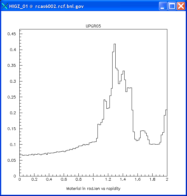
Forward region: the FST and the IGT ONLY:
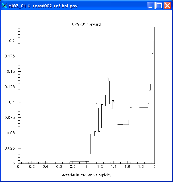
Below, we plot the material for each individual detector, excluding the forward region to reduce ambiguity.
SSD:
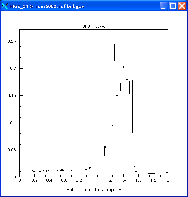
IST:
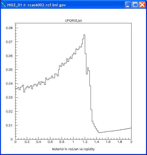
HPD:
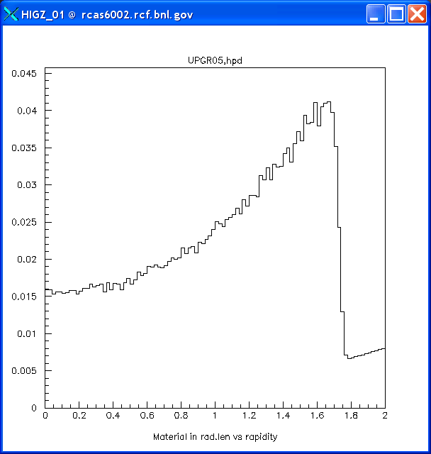
HFT:
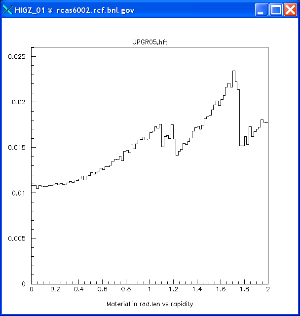
Event Filtering
The attached PDF describes event filtering in the STAR framework.
Event Generators
Event Generator Framework- StarPrimaryMaker -- Main steering class for event generation
- StarGenerator -- Base class (abstract) for interface to event generators
- StarGenEvent -- Base class for event records
- StarGenPPEvent -- Implementation of a generic PP event record
- StarGenEPEvent -- Implementation of a generic EP event record
- StarGenAAEvent -- Implementation of a generic AA event record
- StarGenEAEvent -- Future implementation of a generic EA event record
- StarGenParticle -- Representation of a particle in the STAR event record
- StarParticleData -- "Database" class holding particle data used in simulation
$ cvs co StRoot/StarGenerator/macros
- starsim.pythia6.C
- starsim.pythia8.C
- starsim.hijing.C
- starsim.herwig.C
- starsim.pepsi.C
- starsim.starlight.C
- starsim.kinematics.C
$ ln -s StRoot/StarGenerator/macros/starsim.pythia8.C starsim.C
$ root4star -q -b starsim.C\(100\)
This will generate two files. A standard "fzd" file, which can be reconstructed using the big "full" chain (bfc.C). And a root file, containing a TTree expressing the event record for the generated events.
The new Event Record
The event-wise and particle-wise information from event generators is saved in a ROOT/TTree. The TTree can be read in in sync with the MuDst when you perform your analysis. The ID truth values in the reconstructed tracks in the MuDst can be compared to the primary key of the tracks in the event record to identify generator tracks which were reconstructed by the tracker.
The event record can be browsed using the standard ROOT ttree viewer. Example for pythia 8:
root [0] TFile::Open("pythia8.starsim.root")
root [1] genevents->StartViewer()
root [2] genevents->Draw("mMass","mStatus>0")
The event record contains both particle-wise and event-wise information. For the definitions of different quantities, see the documentation provided in the StarGenEvent links above.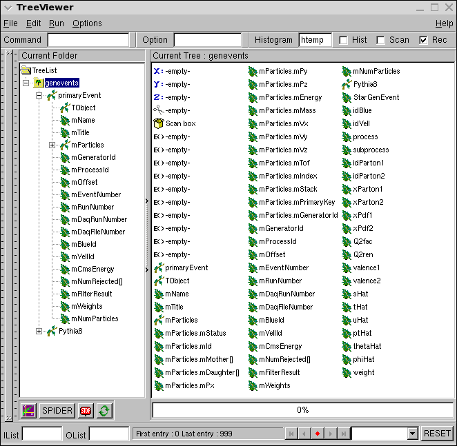
Adding a new Generator
Event generators are responsible for creating the final state particles which are fed out to GEANT for simulation. They can be as simple as particle guns, shooting individual particles along well defined trajectories, or complex hydrodynamical models of heavy-ion collisions. Regardless of the complexities of the underlying physical model, the job of an event generator in the STAR framework is to add particles to an event record. In this document we will describe the steps needed to add a new event generator to the STAR framework. The document will be divided into three sections: (1) An overview, presenting the general steps which are required; (2) A FORtran-specific HOWTO, providing guidance specific to the problem of interfacing FORtran with a C++ application; and (3) A document describing the STAR event record.Contents:
1.0 Integrating Event Generators
2.0 Integrating FORtran Event Generators
3.0 The STAR Event Record
1.0 Integrating Event Generators
The STAR Event Generator Framework implements several C++ classes which facilitate the integration of FORtran and C++ event generators with the STAR simulation code. The code is available in the CVS repository and can be checked out as
$ cvs co StRoot/StarGeneratorAfter checking out the generator area you will note that the code is organized into several directories, containing both CORE packages and concrete event generators. Specifically:
StarGenerator/BASE -- contains the classes implementing the STAR interface to event generators
StarGenerator/EVENT -- contains the classes implementing the STAR event record
StarGenerator/UTIL -- contains random number generator base class and particle data
StarGenerator/TEST -- contains test makers used for validating the event generators
The concrete event generators (at the time this document was assembled) include
StarGenerator/Hijing1_383
StarGenerator/Pepsi
StarGenerator/Pythia6_4_23
StarGenerator/Pythia8_1_62
1.1 Compiling your Generator
Your first task in integrating a new event generator is to create a directory for it under StarGenerator, and get your code to compile. You should select a name for your directory which includes the name and version of your event generator. It should also be CamelCased... MyGenerator1_2_3, for example. (Do not select a name which is ALL CAPS, as this has a special meaning for compilation). Once you have your directory, you can begin moving your source files into the build area. In general, we would like to minimize the number of edits to the source code to make it compile. But you may find that you need to reorganize the directory structure of your code to get it to compile under cons. (For certain, if your FORtran source ends in ".f" you will need to rename the file to ".F", and if your C++ files end in ".cpp" or ".cc", you may need to rename to ".cxx".)
1.2 Creating your Interface
Ok. So the code compiles. Now we need to interface the event generation machinery with the STAR framework. This entails several things. First, we need to expose the configuration of the event generator so that the end user can generate the desired event sample. We must then initialize the concrete event generator at the start of the run, and then exercise the event generation machinery on each and every event. Finally, we need to loop over all of the particles which were created by the event generator and push them onto the event record so that they are persistent (i.e. the full event can be analyzed at a later date) and so that the particles are made available to the Monte Carlo application for simulation.
The base class for all event generator interfaces is StarGenerator.
Taking a quick look at the code, we see that there are several "standard" methods defined for configuring an event generator:
- SetBlue( ... ) -- Sets the blue beam particle, e.g. proton
- SetYell( ... ) -- Sets the yellow beam particle, e.g. Au
- SetFrame( ... ) -- Sets the reference frame, e.g. CMS
You may need to implement additional methods in order to expose the configuration of your event generator. You should, of course, do this.
The two methods which StarGenerator requires you to implement are Init() and Generate(). These methods will respectively be called at the start of each run, and during each event.
Init() is responsible for initializing the event generator. In this method, you should pass any of the configuration information on to your concrete event generator. This may be through calls to subroutines in your event generator, or by setting values in common blocks. However this is done, this is the place to do it.
Generate() will be called on every single event during the run. This is where you should exercise the generation machinery of your event generator. Every event generator handles this differently, so you will need to consult your manual to figure out the details.
Once Generate() has been called, you are ready to fill the event record. The event record consists of two parts: (1) the particle record, and (2) the event-wise information describing the physical interaction being simulated. At a minimum, you will need to fill the particle-wise information. For more details, see The STAR Event Record below.
2.0 Integrating FORtran Event Generators
Interfacing a FORtran event generator with ROOT involves (three) steps:
1. Interface the event generator's common blocks (at least the ones which we need to use) to C++
2. Map those common blocks onto C++ structures
3. Expose the C++ structures representing the common blocks to ROOT so that users may modify / access their contents
Let's look at the pythia event generator for a concrete example.
If you examine the code in StRoot/StarGenerator/Pythia6_4_23/ there is a FORtran file named address.F. Open that up in your favorite editor and have a look... You'll see several functions defined. The first one is address_of_pyjets. In it we declare the PYJETS common block, essentially just cutting and pasting the delcaration from the pythia source code in the same directory.
Next we need to describe the memory layout to C++. This is done in the file Pythia6.h. Each common block setup in address.F has a corresponding structure defined in this header file. So, let's take a look at the setup for the PyJets common block:
First, notice the first line where we call the c-preprocessor macro "F77_NAME". This line handles, in a portable way, the different conventions between FORtran and C++ compilers, when linking together object codes.
Next, let's discuss "memory layout". In this section of the code we map the FORtran memory onto a C-structure. Every variable in the common block should be declared in the same order in the C struct as it was declared in FORtran, and with the corresponding C data type. These are:
INTEGER          --> Int_t
REAL             --> Float_t
REAL *4          --> Float_t
REAL *8          --> Double_t
DOUBLE PRECISION --> Double_t
You probably noticed that there are two differences with the way we have declared the arrays. First, the arrays all were declared with an "_" in front of their name. This was a choice on my part, which I will explain in a moment. The important thing to notice right now is that the indicies on the arrays are reversed, compared to their declarion in FORtran. "INTEGER K(4000,5)" in FORtran becomes "Int_t _k[5][4000]" in C++. The reason for this is that C++ and FORtran represent arrays differently in memory. It is important to keep these differences in mind when mapping the memory of a FORtran common block --
1) The indices in the arrays will always be reversed between FORtran and C -- A(10,20,30) in FORtran becomes A[30][20][10] in C.
2) FORtran indices (by default) start from 1, C++ (always) from 0 -- i.e. B(1) in FORtran would be B[0] in C.
3) FORtran indices may start from any value. An array declared as D(-10:10) would be declared in C as D[21], and D(-10) in FORtran is D[0] in C.
What about the underscore?
We need to make some design choices at this point. Specifically, how do we expose the common blocks to the end user? Do we want the end user to deal with the differences in C++ and FORtran, or do we want to provide a mechanism by which the FORtran behavior (i.e. count from 1, preserve the order of indices) can be emulated.
My preference is to do the latter -- provide the end user functions which emulate the behavior of the FORtran arrays, because these arrays are what is documented in the event generator's manual. This will minimize the likelyhood that the end user will make mistakes in configuring t he event generator.
So we have created a c-struct which describes how the common block's memory is laid out, and we have defined a function in the FORtran library which returns the location of the memory address of the common block. Now we need to expose that function to C++. To do that, we need to declare a prototype of the function. There are two things we need to do.
First, we need to define the name of the subroutine in a portable way. This is done using a macro defined in #include "StarCallf77.h" --
#define address_of_pyjets F77_NAME( address_of_pyjets, ADDRESS_OF_PYJETS )
Next we need to declare to C++ that address_of_pyjets can be found in an external library, and will return a pointer to the PyJets_t structure
extern "C" PyJets_t *address_of_pyjets();
Now we are almost done. We need to add a function in our generator class which returns a pointer (or reference) to the common blocks, and we need to add PyJets_t to the ROOT dictionary... In MyGeneratorLinkDef.h, add the line
#pragma link C++ struct PyJets_t+;
Finally, you need to expose the FORtran subroutines to C++. Again, take a look at the code in Pythia6.h and Pythia6.cxx. In the header we declare wrapper functions around the FORtran subroutines, and in the implementation file we expose the FORtran subroutines to C++.
Our first step is declaring the prototypes of the subroutines and implementing the C++ infterface. Consider the SUBROUTINE PYINIT in pythia, which initializes the event generator. In FORtran it is declared as
SUBROUTINE PYINIT(FRAME,BEAM,TARGET,WIN)
IMPLICIT DOUBLE PRECISION(A-H, O-Z)
IMPLICIT INTEGER(I-N)
...
CHARACTER*(*) FRAME,BEAM,TARGET
So the variables FRAME, BEAM and TARGET are declared as character variables, and WIN is implicitly a double precision variable.
There are several webpages which show how to interface fortran and c++, e.g. http://www.yolinux.com/TUTORIALS/LinuxTutorialMixingFortranAndC.html
It is really a system-dependent thing. We're keeping it simple and only supporting Linux.
#define pyinit F77_NAME(pyinit,PYINIT) /* pythia initialization */
extern "C" void type_of_call pyinit( const char *frame,
const char *beam,
const char *targ,
double *ener,
int nframe,
int nbeam,
int ntarg );
So there's three character varaibles declared: frame, beam and targ. These correspond to the character variables on the FORtran side. Also there's a double precision variable ener... this is WIN. But then there are three integer variables nframe, nbeam and ntarg. FORtran expects to get the size of the character variables when the subroutine is called, and it gets them after the last arguements in the list.
Again, we would like to hide this from the end user... so I like to define wrapper functions such as
#include <string>
void PyInit( string frame, string blue, string yellow, double energy )
{
pyinit( frame.c_str(), blue.c_str(), yellow.c_str(), &energy,
frame.size(),
blue.size(),
yellow.size() );
}
3.0 The STAR Event Record
List of Event Generators
Event generators currently integrated into starsim using the root4star framework (11/29/12):
- Pythia 6.4.23
- Pythia 8.1.62
- Hijing 1.383
- Herwig 6.5.20
- StarLight
- Pepsi
To run, checkout StRoot/StarGenerator/macros and modify the appropriate example ROOT macro for your purposes.
Event generators currently implemented in the starsim framework (11/29/12):
- Hijing 1.381
- Hijing 1.382
- Pythia 6.2.05
- Pythia 6.2.20
- Pythia 6.4.10
- Pythia 6.4.22
- Pythia 6.4.26
- StarLight (fortran)
The STAR Event Record
Geometry Tags
Geometry Tag y2000
CaveGeo PipeGeo UpstGeo SvttGeo tpcegeo
BtofGeo2 CalbGeo ZcalGeo MagpGeo
Geometry Tag y2001
CaveGeo PipeGeo UpstGeo SvttGeo1 tpcegeo
FtpcGeo SupoGeo1 BtofGeo2 VpddGeo CalbGeo
richgeo EcalGeo ZcalGeo MagpGeo
Geometry Tag y2002
CaveGeo PipeGeo UpstGeo SvttGeo tpcegeo
FtpcGeo SupoGeo BtofGeo2 VpddGeo CalbGeo
richgeo BbcmGeo fpdmgeo ZcalGeo MagpGeo
Geometry Tag y2003
CaveGeo PipeGeo UpstGeo SvttGeo tpcegeo
FtpcGeo SupoGeo BtofGeo2 VpddGeo CalbGeo
EcalGeo BbcmGeo fpdmgeo ZcalGeo MagpGeo
Geometry Tag y2003x
CaveGeo PipeGeo UpstGeo SvttGeo2 tpcegeo
FtpcGeo SupoGeo1 BtofGeo2 VpddGeo CalbGeo
EcalGeo BbcmGeo fpdmgeo ZcalGeo MagpGeo
PhmdGeo
Geometry Tag y2004a
CaveGeo PipeGeo UpstGeo SvttGeo3 tpcegeo
FtpcGeo SupoGeo1 BtofGeo2 VpddGeo CalbGeo1
EcalGeo BbcmGeo FpdmGeo1 ZcalGeo MagpGeo
SisdGeo PhmdGeo
Geometry Tag y2004c
CaveGeo PipeGeo UpstGeo SvttGeo4 TpceGeo1
FtpcGeo SupoGeo1 BtofGeo2 VpddGeo CalbGeo1
EcalGeo BbcmGeo FpdmGeo1 ZcalGeo MagpGeo
SisdGeo1 PhmdGeo
Geometry Tag y2004y
CaveGeo PipeGeo UpstGeo SvttGeo4 TpceGeo1
FtpcGeo1 SupoGeo1 FtroGeo BtofGeo2 VpddGeo
CalbGeo EcalGeo BbcmGeo FpdmGeo1 ZcalGeo
MagpGeo SisdGeo2 PhmdGeo
Geometry Tag y2005
CaveGeo PipeGeo UpstGeo SvttGeo3 tpcegeo
FtpcGeo1 SupoGeo1 FtroGeo BtofGeo2 VpddGeo
CalbGeo1 EcalGeo BbcmGeo FpdmGeo1 ZcalGeo
MagpGeo SisdGeo2 PhmdGeo
Geometry Tag y2005b
CaveGeo PipeGeo UpstGeo SvttGeo4 TpceGeo1
FtpcGeo1 SupoGeo1 FtroGeo BtofGeo2 VpddGeo
CalbGeo1 EcalGeo BbcmGeo FpdmGeo1 ZcalGeo
MagpGeo SisdGeo2 PhmdGeo
Geometry Tag y2005f
CaveGeo PipeGeo UpstGeo SvttGeo6 TpceGeo1
FtpcGeo1 SupoGeo1 FtroGeo BtofGeo4 VpddGeo
CalbGeo2 EcalGeo BbcmGeo FpdmGeo1 ZcalGeo
MagpGeo SisdGeo6 PhmdGeo
Geometry Tag y2005g
CaveGeo PipeGeo UpstGeo SvttGeo11 TpceGeo1
FtpcGeo1 SupoGeo1 FtroGeo BtofGeo4 VpddGeo
CalbGeo2 EcalGeo BbcmGeo FpdmGeo1 ZcalGeo
MagpGeo SisdGeo6 PhmdGeo
Geometry Tag y2005h
CaveGeo PipeGeo UpstGeo SvttGeo11 tpcegeo3
FtpcGeo1 SupoGeo1 FtroGeo BtofGeo4 VpddGeo
CalbGeo2 EcalGeo BbcmGeo FpdmGeo1 ZcalGeo
MagpGeo SisdGeo6 PhmdGeo
Geometry Tag y2005i
CaveGeo PipeGeo UpstGeo SvttGeo11 tpcegeo3
FtpcGeo1 SupoGeo1 FtroGeo BtofGeo4 VpddGeo
CalbGeo2 EcalGeo6 BbcmGeo FpdmGeo1 ZcalGeo
MagpGeo SisdGeo6 PhmdGeo
Geometry Tag y2006
CaveGeo PipeGeo UpstGeo SvttGeo6 TpceGeo2
FtpcGeo1 SupoGeo1 FtroGeo BtofGeo4 VpddGeo
CalbGeo1 EcalGeo BbcmGeo FpdmGeo1 ZcalGeo
MagpGeo SisdGeo3 MutdGeo PhmdGeo
Geometry Tag y2006c
CaveGeo PipeGeo UpstGeo SvttGeo6 TpceGeo2
FtpcGeo1 SupoGeo1 FtroGeo BtofGeo4 VpddGeo
CalbGeo2 EcalGeo BbcmGeo FpdmGeo2 ZcalGeo
MagpGeo SisdGeo6 MutdGeo
Geometry Tag y2006g
CaveGeo PipeGeo UpstGeo SvttGeo11 TpceGeo2
FtpcGeo1 SupoGeo1 FtroGeo BtofGeo4 VpddGeo
CalbGeo2 EcalGeo BbcmGeo FpdmGeo2 ZcalGeo
MagpGeo SisdGeo6 MutdGeo
Geometry Tag y2006h
CaveGeo PipeGeo UpstGeo SvttGeo11 tpcegeo3
FtpcGeo1 SupoGeo1 FtroGeo BtofGeo4 VpddGeo
CalbGeo2 EcalGeo6 BbcmGeo FpdmGeo2 ZcalGeo
MagpGeo SisdGeo6 MutdGeo
Geometry Tag y2007
CaveGeo PipeGeo UpstGeo SvttGeo6 TpceGeo2
FtpcGeo1 SupoGeo1 FtroGeo BtofGeo5 VpddGeo2
CalbGeo2 EcalGeo BbcmGeo FpdmGeo3 ZcalGeo
MagpGeo SisdGeo6 MutdGeo PhmdGeo
Geometry Tag y2007g
CaveGeo PipeGeo UpstGeo SvttGeo11 TpceGeo2
FtpcGeo1 SupoGeo1 FtroGeo BtofGeo5 VpddGeo2
CalbGeo2 EcalGeo BbcmGeo FpdmGeo3 ZcalGeo
MagpGeo SisdGeo6 MutdGeo PhmdGeo
Geometry Tag y2007h
CaveGeo PipeGeo UpstGeo SvttGeo11 tpcegeo3
FtpcGeo1 SupoGeo1 FtroGeo BtofGeo5 VpddGeo2
CalbGeo2 EcalGeo BbcmGeo FpdmGeo3 ZcalGeo
MagpGeo SisdGeo6 MutdGeo PhmdGeo
Geometry Tag y2008
CaveGeo PipeGeo UpstGeo TpceGeo2 FtpcGeo1
SupoGeo1 FtroGeo BtofGeo6 VpddGeo2 CalbGeo2
EcalGeo BbcmGeo FpdmGeo3 ZcalGeo MagpGeo
MutdGeo3
Geometry Tag y2008a
CaveGeo PipeGeo UpstGeo SconGeo TpceGeo2
FtpcGeo1 SupoGeo1 FtroGeo BtofGeo6 VpddGeo2
CalbGeo2 EcalGeo BbcmGeo FpdmGeo3 ZcalGeo
MagpGeo MutdGeo3
Geometry Tag y2008b
CaveGeo PipeGeo UpstGeo SconGeo tpcegeo3
FtpcGeo1 SupoGeo1 FtroGeo BtofGeo6 VpddGeo2
CalbGeo2 EcalGeo6 BbcmGeo FpdmGeo3 ZcalGeo
MagpGeo MutdGeo3
Geometry Tag y2008c
CaveGeo PipeGeo UpstGeo SconGeo tpcegeo3
FtpcGeo1 SupoGeo1 FtroGeo BtofGeo7 VpddGeo2
CalbGeo2 EcalGeo6 BbcmGeo FpdmGeo3 ZcalGeo
MagpGeo MutdGeo3
Geometry Tag y2008d
CaveGeo PipeGeo UpstGeo SconGeo tpcegeo3
FtpcGeo1 SupoGeo1 FtroGeo BtofGeo7 VpddGeo2
CalbGeo2 EcalGeo6 BbcmGeo FpdmGeo3 ZcalGeo
MagpGeo MutdGeo3
Geometry Tag y2008e
CaveGeo PipeGeo UpstGeo SconGeo tpcegeo3
FtpcGeo1 SupoGeo1 FtroGeo BtofGeo7 VpddGeo2
CalbGeo2 EcalGeo6 BbcmGeo FpdmGeo3 ZcalGeo
MagpGeo MutdGeo3
Geometry Tag y2009
EcalGeo PipeGeo FpdmGeo3 BtofGeo6 VpddGeo2
FtpcGeo1 FtroGeo MutdGeo3 TpceGeo3a CalbGeo2
SconGeo UpstGeo ZcalGeo CaveGeo MagpGeo
BbcmGeo
Geometry Tag y2009a
EcalGeo6 PipeGeo FpdmGeo3 BtofGeo6 VpddGeo2
FtpcGeo1 FtroGeo MutdGeo3 TpceGeo3a CalbGeo2
SconGeo UpstGeo ZcalGeo CaveGeo MagpGeo
BbcmGeo
Geometry Tag y2009b
EcalGeo6 PipeGeo FpdmGeo3 BtofGeo6 VpddGeo2
FtpcGeo1 FtroGeo MutdGeo3 TpceGeo3a CalbGeo2
SconGeo UpstGeo ZcalGeo CaveGeo MagpGeo
BbcmGeo
Geometry Tag y2009c
EcalGeo6 PipeGeo FpdmGeo3 BtofGeo7 VpddGeo2
FtpcGeo1 FtroGeo MutdGeo3 TpceGeo3a CalbGeo2
SconGeo UpstGeo ZcalGeo CaveGeo MagpGeo
BbcmGeo
Geometry Tag y2009d
EcalGeo6 PipeGeo FpdmGeo3 BtofGeo7 VpddGeo2
FtpcGeo1 FtroGeo MutdGeo3 TpceGeo3a CalbGeo2
SconGeo UpstGeo ZcalGeo CaveGeo MagpGeo
BbcmGeo
Geometry Tag y2010
EcalGeo6 PipeGeo FpdmGeo3 BtofGeo6 VpddGeo2
FtpcGeo1 FtroGeo MutdGeo3 TpceGeo3a CalbGeo2
SconGeo PhmdGeo UpstGeo ZcalGeo CaveGeo
MagpGeo BbcmGeo
Geometry Tag y2010a
EcalGeo6 PipeGeo FpdmGeo3 BtofGeo6 VpddGeo2
FtpcGeo1 FtroGeo MutdGeo3 TpceGeo3a CalbGeo2
SconGeo PhmdGeo UpstGeo ZcalGeo CaveGeo
MagpGeo BbcmGeo
Geometry Tag y2010b
EcalGeo6 PipeGeo FpdmGeo3 BtofGeo7 VpddGeo2
FtpcGeo1 FtroGeo MutdGeo3 TpceGeo3a CalbGeo2
SconGeo PhmdGeo UpstGeo ZcalGeo CaveGeo
MagpGeo BbcmGeo
Geometry Tag y2010c
EcalGeo6 PipeGeo FpdmGeo3 BtofGeo7 VpddGeo2
FtpcGeo1 FtroGeo MutdGeo3 TpceGeo3a CalbGeo2
SconGeo PhmdGeo UpstGeo ZcalGeo CaveGeo
MagpGeo BbcmGeo
Geometry Tag y2011
EcalGeo6 PipeGeo FpdmGeo3 BtofGeo7 VpddGeo2
FtpcGeo1 FtroGeo MutdGeo4 TpceGeo3a CalbGeo2
SconGeo PhmdGeo UpstGeo ZcalGeo CaveGeo
MagpGeo BbcmGeo
Geometry Tag y2011a
EcalGeo6 PipeGeo FpdmGeo3 BtofGeo7 VpddGeo2
FtpcGeo1 FtroGeo MutdGeo4 TpceGeo3a CalbGeo2
SconGeo PhmdGeo UpstGeo ZcalGeo CaveGeo
MagpGeo BbcmGeo
Geometry Tag y2012
EcalGeo6 PipeGeo FpdmGeo3 BtofGeo7 VpddGeo2
MutdGeo4 TpceGeo3a CalbGeo2 UpstGeo ZcalGeo
CaveGeo MagpGeo BbcmGeo FgtdGeo3 IdsmGeo1
Geometry Tag y2012a
EcalGeo6 PipeGeo FpdmGeo3 BtofGeo7 VpddGeo2
MutdGeo4 TpceGeo3a CalbGeo2 UpstGeo ZcalGeo
CaveGeo MagpGeo BbcmGeo FgtdGeo3 IdsmGeo1
Geometry Tag y2012b
EcalGeo6 PipeGeo FpdmGeo3 BtofGeo7 VpddGeo2
MutdGeo4 TpceGeo3a CalbGeo2 UpstGeo ZcalGeo
CaveGeo MagpGeo BbcmGeo FgtdGeo3 IdsmGeo1
Geometry Tag y2013
EcalGeo6 PipeGeo2 FpdmGeo3 BtofGeo8 VpddGeo2
MutdGeo4 TpceGeo3a CalbGeo2 UpstGeo ZcalGeo
CaveGeo MagpGeo BbcmGeo FgtdGeo3 IdsmGeo1
PixlGeo5 PxstGeo1 DtubGeo1
Geometry Tag y2013_1
EcalGeo6 PipeGeo2 FpdmGeo3 BtofGeo8 VpddGeo2
MutdGeo4 TpceGeo3a CalbGeo2 UpstGeo ZcalGeo
CaveGeo MagpGeo BbcmGeo FgtdGeo3 IdsmGeo1
PixlGeo5 PxstGeo1 DtubGeo1
Geometry Tag y2013_2
EcalGeo6 PipeGeo2 FpdmGeo3 BtofGeo8 VpddGeo2
MutdGeo4 TpceGeo3a CalbGeo2 UpstGeo ZcalGeo
CaveGeo MagpGeo BbcmGeo FgtdGeo3 IdsmGeo1
PxstGeo1
Geometry Tag y2013_1x
EcalGeo6 PipeGeo2 FpdmGeo3 BtofGeo8 VpddGeo2
MutdGeo4 TpceGeo3a CalbGeo2 UpstGeo ZcalGeo
CaveGeo2 MagpGeo BbcmGeo FgtdGeo3 IdsmGeo1
PixlGeo5 PxstGeo1 DtubGeo1
Geometry Tag y2013x
EcalGeo6 PipeGeo2 FpdmGeo3 BtofGeo8 VpddGeo2
MutdGeo4 TpceGeo3a CalbGeo2 UpstGeo ZcalGeo
CaveGeo2 MagpGeo BbcmGeo FgtdGeo3 IdsmGeo1
PixlGeo5 PxstGeo1 DtubGeo1
Geometry Tag y2013_2x
EcalGeo6 PipeGeo2 FpdmGeo3 BtofGeo8 VpddGeo2
MutdGeo4 TpceGeo3a CalbGeo2 UpstGeo ZcalGeo
CaveGeo2 MagpGeo BbcmGeo FgtdGeo3 IdsmGeo1
PxstGeo1
Geometry Tag dev14
EcalGeo6 PipeGeo1 FpdmGeo3 BtofGeo7 VpddGeo2
MutdGeo4 TpceGeo3a CalbGeo2 CaveGeo BbcmGeo
SisdGeo7 FgtdGeo3 IdsmGeo1 PixlGeo4 IstdGeo0
PxstGeo1
Geometry Tag complete
EcalGeo6 PipeGeo FpdmGeo3 BtofGeo7 VpddGeo2
MutdGeo4 TpceGeo3a CalbGeo2 PhmdGeo UpstGeo
ZcalGeo CaveGeo MagpGeo BbcmGeo FgtdGeo3
IdsmGeo1
Geometry Tag devT
EcalGeo6 PipeGeo FpdmGeo3 BtofGeo7 VpddGeo2
MutdGeo4 CalbGeo2 UpstGeo ZcalGeo CaveGeo
MagpGeo BbcmGeo FgtdGeo3 IdsmGeo1 FsceGeo
EiddGeo TpcxGeo1
Geometry Tag eStar2
EcalGeo6 PipeGeo FpdmGeo3 BtofGeo7 VpddGeo2
MutdGeo4 CalbGeo2 UpstGeo ZcalGeo CaveGeo
MagpGeo BbcmGeo FgtdGeoV IdsmGeo1 FsceGeo
EiddGeo TpcxGeo2
Material Budget Y2013
Material budget in the Y2013 (X) geometry. The top left plots number of radiation lengths encounted by a straight track at the given eta, phi. The top right (bottom left) compares the ROOT and STARSIM geometries generated by AgML plotted vs phi (eta). These are averaged over the other variable. ROOT geometry in black, STARSIM in red. The bottom right shows the difference in ROOT - STARSIM geometries vs phi and eta. Less than 0.01 radiation lengths difference found integrated over the entire cave.
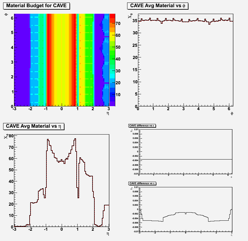
Attached are material budget plots and differences for major subsystems. Each PDF contains the material budget plots displaying number of radiation lengths averaged over all phi for the ROOT (left) and STARSIM (right) geometries created by AgML. The material difference plot is as described above.
Miscellaneous production scripts
This page has been created with the purpose to systematize the various scripts currently used in the Monte Carlo production and testing. The contents will be updated as needed, however the codes are presumed to be correct and working at any given time.
Jobs catalog
When running on rcas, we typically use a legacy csh script named "alljobs". It parses the job configuration file named "catalog" and dispatches a single job on the target node, which can be an interactive node if run interactively, or a batch node if submitted to a queue. The alljobs script expects to see the following directory structure: a writeable directory with the name of the dataset being produced, and directly under it, a writeable "log" directory, in which it would deposit the so-called token files, which serve two purposes:
- help in sequential numbering of the output files
- in case of multiple input files (such as Hijing event files) allow to map N files to M jobs, thus managing the workload
The catalog file is effectively a table, in white-space separated format. Each line begins with the dataset name which is a three-letter acronym of the site name (and thus either rcf or pds) followed by a 4-digit serial number of the set. The alljobs script expects to find a directory named identically to the dataset, under the "job directory", which in the current version of the script is hardcoded as /star/simu/simu/gstardata. This, of course, can be improved or changed.
The last field in each entry is used to construct the so-called tag, which plays an important role: it effectively defined the location of the Monte Carlo data in the HPSS, when the data is sunk there (this is done by a separate script). In addition, it also defines keys for the entries in the FileCatalog (reconstructed data). The alljobs script creates a file of zero length, with a name which is a period-separated catenation of the word "tag" and the contents of the last column in the line.
Here are the contents of the catalog file as it existed from the late 1990-s to the end of 2006
rcf0101 auau200/nexus/default/central            evgen.*.nt   auau200.nexus.default.b0_3.year_1h.hadronic_on
rcf0105 auau200/nexus/default/minbias            evgen.*.nt   auau200.nexus.default.minbias.year_1h.hadronic_on
pds0101 auau200/vni/default/central              evgen.*.nt   auau200.vni.default.b0_3.year_1h.hadronic_on
pds0102 auau200/vni/default/central              evgen.*.nt   auau200.vni.default.b0_3.year_1h.hadronic_on
pds0103 auau200/vni/default/central              evgen.*.nt   auau200.vni.default.b0_3.year_1h.hadronic_on
pds0104 auau200/vni/default/central              evgen.*.nt   auau200.vni.default.b0_3.year_1h.hadronic_on
rcf0096 auau200/vni/default/central              evgen.*.nt   auau200.vni.default.b0_3.year_1h.hadronic_on

pds0105 auau200/mevsim/vanilla_trigger/central   evgen.*.nt   auau200.mevsim.vanilla.trigger.year_1h.hadronic_on
rcf0097 auau200/mevsim/vanilla_resonance/central evgen.*.nt   auau200.mevsim.vanilla.resonance.year_1h.hadronic_on
rcf0098 auau200/mevsim/vanilla_trigger/central   evgen.*.nt   auau200.mevsim.vanilla.trigger.year_1h.hadronic_on
rcf0095 auau200/mevsim/vanilla_flow/central      evgen.*.nt   auau200.mevsim.vanilla.flow.year_1h.hadronic_on
rcf0099 auau200/mevsim/vanilla_fluct/central     evgen.*.nt   auau200.mevsim.vanilla.fluct.year_1h.hadronic_on
rcf0102 auau200/mevsim/vanilla/central           evgen.*.nt   auau200.mevsim.vanilla.central.year_1h.hadronic_on
rcf0103 auau200/mevsim/vanilla/central           evgen.*.nt   auau200.mevsim.vanilla.central.year_1h.hadronic_on
rcf0104 auau200/mevsim/vanilla_flow/central      evgen.*.nt   auau200.mevsim.vanilla.flow.year_1h.hadronic_on
rcf0100 auau200/mevsim/cascade/central           evgen.*.nt   auau200.mevsim.cascade.central.year_1h.hadronic_on

rcf0106 auau200/hbt/default/peripheral           evgen.*.nt   auau200.hbt.default.peripheral.year_1h.hadronic_on
rcf0107 auau200/hbt/default/midperipheral        evgen.*.nt   auau200.hbt.default.midperipheral.year_1h.hadronic_on
rcf0108 auau200/hbt/default/middle               evgen.*.nt   auau200.hbt.default.middle.year_1h.hadronic_on
rcf0109 auau200/hbt/default/midcentral           evgen.*.nt   auau200.hbt.default.midcentral.year_1h.hadronic_on
rcf0110 auau200/hbt/default/central              evgen.*.nt   auau200.hbt.default.central.year_1h.hadronic_on

rcf0111 none                                    hijing.*.xdf  auau200.hijing.b0_3_jetq_on.jet05.year_1h.hadronic_on
rcf0112 none                                    hijing.*.xdf  auau200.hijing.b0_3_jetq_off.jet05.year_1h.hadronic_on
rcf0113 none                                    hijing.*.xdf  auau200.hijing.b8_15_jetq_on.jet05.year_1h.hadronic_on
rcf0114 none                                    hijing.*.xdf  auau200.hijing.b8_15_jetq_off.jet05.year_1h.hadronic_on
rcf0115 none                                    hijing.*.xdf  auau200.hijing.b0_3_jetq_on.jet05.year_1h.hadronic_on
rcf0116 none                                    hijing.*.xdf  auau200.hijing.b0_3_jetq_off.jet05.year_1h.hadronic_on
rcf0117 none                                    hijing.*.xdf  auau200.hijing.b8_15_jetq_on.jet05.year_1h.hadronic_on
rcf0118 none                                    hijing.*.xdf  auau200.hijing.b8_15_jetq_off.jet05.year_1h.hadronic_on
rcf0119 none                                    hijing.*.xdf  pau200_hijing_b0_7_jet15_year_1h.hadronic_on
rcf0120 none                                    hijing.*.xdf  pau200_hijing_b0_7_gam15_year_1h_hadronic_on

rcf0121 pec/dtunuc                               dtu*.xdr     auau200.dtunuc.two_photon.none.year_1h.hadronic_on
rcf0122 pec/starlight                  starlight_vmeson_*.t   auau200.starlight.vmeson.none.year_1h.hadronic_on
rcf0123 pec/starlight                  starlight_2gamma_*.nt  auau200.starlight.2gamma.none.year_1h.hadronic_on
rcf0124 pec/hemicosm                             events.txt   auau200.hemicosm.default.none.year_1h.hadronic_on

rcf0125 pec/dtunuc                               dtu*.xdr     auau200.dtunuc.two_photon.halffield.year_1h.hadronic_on
rcf0126 pec/starlight                  starlight_vmeson_*.t   auau200.starlight.vmeson.halffield.year_1h.hadronic_on
rcf0127 pec/starlight                  starlight_2gamma_*.t   auau200.starlight.2gamma.halffield.year_1h.hadronic_on

rcf0131 pec/beamgas                            venus.h.*.nt   auau200.hijing.beamgas.hydrogen.year_1h.hadronic_on
rcf0132 pec/beamgas                            venus.n.*.nt   auau200.hijing.beamgas.nitrogen.year_1h.hadronic_on

rcf0139 none                                     hijev.inp    auau128.hijing.b0_12.halffield.year_1e.hadronic_on
rcf0140 none                                     hijev.inp    auau128.hijing.b0_3.halffield.year_1e.hadronic_on

rcf0141 auau200/strongcp/broken/eb_400_90        evgen.*.nt   auau200.strongcp.broken.eb-400_90.year_1h.hadronic_on
rcf0142 auau200/strongcp/broken/eb_400_00        evgen.*.nt   auau200.strongcp.broken.eb-400_00.year_1h.hadronic_on
rcf0143 auau200/strongcp/broken/lr_eb_400_90     evgen.*.nt   auau200.strongcp.broken.lr_eb_400_90.year_1h.hadronic_on

rcf0145 none                                  hijev.inp    auau130.hijing.b0_3.jet05.year_1h.halffield.hadronic_on
rcf0146 none                                  hijev.inp    auau130.hijing.b0_15.default.year_1h.halffield.hadronic_on
rcf0147 none                                  hijev.inp    auau130.hijing.b0_3.default.year_1e.halffield.hadronic_on
rcf0148 none                                  hijev.inp    auau130.hijing.b3_6.default.year_1e.halffield.hadronic_on

rcf0151 auau130/mevsim/vanilla_flow/central      evgen.*.nt   auau130.mevsim.vanilla_flow.central.year_1e.hadronic_on
rcf0152 auau130/mevsim/vanilla_trigger/central   evgen.*.nt   auau130.mevsim.vanilla_trigger.central.year_1e.hadronic_on
rcf0153 auau130/mevsim/vanilla_dynamic/central   evgen.*.nt   auau130.mevsim.vanilla_dynamic.central.year_1e.hadronic_on
rcf0154 auau130/mevsim/vanilla_omega/central     evgen.*.nt   auau130.mevsim.vanilla_omega.central.year_1e.hadronic_on
rcf0155 auau130/mevsim/vanilla/central           evgen.*.nt   auau130.mevsim.vanilla.central.year_1e.hadronic_on
rcf0156 auau130/nexus/default/central            evgen.*.nt   auau130.nexus.default.b0_3.year_1e.hadronic_on

rcf0159 rqmd                                auau_b0-14.*.cwn  auau200.rqmd.default.b0_14.year_1h.hadronic_on
rcf0160 rqmd                                auau_b0-15.*.cwn  auau200.rqmd.default.b0_15.year_1h.hadronic_on

rcf0161 auau130/mevsim/vanilla_flow/central      evgen.*.nt   auau130.mevsim.vanilla_flow.central.year_1h.hadronic_on
rcf0162 auau130/mevsim/vanilla_trigger/central   evgen.*.nt   auau130.mevsim.vanilla_trigger.central.year_1h.hadronic_on
rcf0163 auau130/mevsim/vanilla_dynamic/central   evgen.*.nt   auau130.mevsim.vanilla_dynamic.central.year_1h.hadronic_on
rcf0164 auau130/mevsim/vanilla_omega/central     evgen.*.nt   auau130.mevsim.vanilla_omega.central.year_1h.hadronic_on
rcf0165 auau130/mevsim/vanilla/central           evgen.*.nt   auau130.mevsim.vanilla.central.year_1h.hadronic_on
rcf0166 auau130/mevsim/vanilla_resonance/central evgen.*.nt   auau130.mevsim.vanilla_resonance.central.year_1h.hadronic_on
pds0167 auau130/mevsim/vanilla_cocktail/central  evgen.*.nt   auau130.mevsim.vanilla_cocktail.central.year_1h.hadronic_on
rcf0168 auau130/mevsim/vanilla_flow/mbias        evgen.*.nt   auau130.mevsim.vanilla_flow.minbias.year_1h.hadronic_on
rcf0169 auau130/mevsim/vanilla_flowb/central     evgen.*.nt   auau130.mevsim.vanilla_flowb.central.year_1h.hadronic_on

rcf0171 auau130/mevsim/vanilla_lambda_antilambda/central evgen.*.nt auau130.mevsim.vanilla_both_lambda.central.year_1h.hadronic_on
rcf0172 auau130/mevsim/vanilla_lambda/central            evgen.*.nt auau130.mevsim.vanilla_lambda.central.year_1h.hadronic_on
rcf0173 auau130/mevsim/vanilla_antilambda/central        evgen.*.nt auau130.mevsim.vanilla_antilambda.central.year_1h.hadronic_on

rcf0181 auau200/mevsim/mdc4/central               evgen.*.nt  auau200.mevsim.mdc4_cocktail.central.year2001.hadronic_on
pds0182 auau200/mevsim/mdc4/central               evgen.*.nt  auau200.mevsim.mdc4_cocktail.central.year2001.hadronic_on

rcf0183 none                                     hijev.inp  auau200.hijing.b0_20.standard.year2001.hadronic_on
rcf0184 none                                     hijev.inp  auau200.hijing.b0_3.standard.year2001.hadronic_on

rcf0190 auau200/mevsim/mdc4_electrons   evgen.*.nt  auau200.mevsim.mdc4_electrons.year2001.hadronic_on

rcf0191 none                                     hijev.inp  auau200.hijing.b0_20.inverse.year2001.hadronic_on
rcf0192 none                                     hijev.inp  auau200.hijing.b0_3.inverse.year2001.hadronic_on
rcf0193 none                                     hijev.inp  dau200.hijing.b0_20.standard.year_2a.hadronic_on

# Maxim has arrived:
# the following two runs had the 1 6 setting for the hard scattering and energy
rcf0194 none                                     hijev.inp  dau200.hijing.b0_20.jet06.year2003.hadronic_on
pds0195 none                                     hijev.inp  dau200.hijing.b0_20.jet06.year2003.hadronic_on
# this one had 1 3
rcf0196 none                                     hijev.inp  dau200.hijing.b0_20.jet03.year2003.hadronic_on
# standard 0 2 setting
rcf0197 none                                     hijev.inp  dau200.hijing.b0_20.jet02.year2003.hadronic_on
# new numbering
rcf1197 none					 hijev.inp  dau200.hijing.b0_20.minbias.year2003.hadronic_on
rcf1198 dau200/hijing_382/b0_20/minbias          evgen.*.nt dau200.hijing_382.b0_20.minbias.year2003.gheisha_on
# dedicated wide Z run
rcf1199 dau200/hijing_382/b0_20/minbias          evgen.*.nt dau200.hijing_382.b0_20.minbias_wideZ.year2003.hadronic_on
# Pythia
rcf1200 none                                     pyth.dat   pp200.pythia6_203.default.minbias.year2003.hadronic_on
# Heavy flavor embedding with full calorimeter
rcf1201 auau200/hijing_382/b0_20/minbias         evgen.*.nt auau200.hijing_382.b0_20.minbias.y2003x.gheisha_on
# Pythia hi Pt>5
rcf1202 none                                     pyth.dat   pp200.pythia6_203.default.pt5.year2003.gheisha_on
# Mevsim fitted to 200GeV AuAu
rcf1203 auau200/mevsim/v2/central_6              evgen.*.nt auau200.mevsim.v2.b0_6.year_1e.gheisha_on
# Mevsim fitted to 200GeV AuAu, different geo
rcf1204 auau200/mevsim/v2/central_6              evgen.*.nt auau200.mevsim.v2.b0_6.year2001.gheisha_on
# Pythia hi Pt>15
rcf1205 none                                     pyth.dat   pp200.pythia6_203.default.pt15.year2003.gheisha_on
# Starsim maiden voyage, with y2004, 62.4 GeV
rcf1206 auau62/hijing_382/b0_20/minbias          evgen.*.nt auau62.hijing_382.b0_20.minbias.y2004.gheisha_on
# 62.4 GeV central
rcf1207 auau62/hijing_382/b0_3/central           evgen.*.nt auau62.hijing_382.b0_3.central.y2004a.gheisha_on
pds1207 auau62/hijing_382/b0_3/central           evgen.*.nt auau62.hijing_382.b0_3.central.y2004a.gheisha_on
# 200 GeV minbias
rcf1208 auau200/hijing_382/b0_20/minbias         evgen.*.nt auau200.hijing_382.b0_20.minbias.y2004a.gheisha_on
# 200 GeV central
rcf1209 auau200/hijing_382/b0_3/central          evgen.*.nt auau200.hijing_382.b0_3.central.y2004a.gheisha_on
# Pythia
rcf1210 none                                     pyth.dat   pp200.pythia6_203.default.minbias.y2004a.gheisha_on
# Pythia Spin group
rcf1211 none                                     pyth.dat   pp200.pythia6_203.default.minbias.y2004x.gheisha_on
# Pythia Spin group
pds1212 none                                     pyth.dat   pp200.pythia6_203.default.pt3.y2004x.gheisha_on
# Pythia Spin group
rcf1213 none                                     pyth.dat   pp200.pythia6_205.default.pt7.y2004x.gheisha_on
# Pythia Spin group
pds1214 none                                     pyth.dat   pp200.pythia6_203.default.pt15.y2004x.gheisha_on
# 200 GeV minbias special D decays
rcf1215 auau200/hijing_382/b0_20/minbias         evgen.*.nt auau200.hijing_382.b0_20.speciald.y2004a.gheisha_on
# 200 GeV minbias copper
rcf1216 cucu200/hijing_382/b0_14/minbias         evgen.*.nt cucu200.hijing_382.b0_14.minbias.y2005x.gheisha_on
# 200 GeV minbias copper test
rcf1217 cucu200/hijing_382/b0_14/minbias         evgen.*.nt cucu200.hijing_382.b0_14.minbias.y2004a.gheisha_on
# 200 GeV central reprise of 1209, smaller diamond
rcf1218 auau200/hijing_382/b0_3/central          evgen.*.nt auau200.hijing_382.b0_3.central.y2004a.gheisha_on
# Pythia Special 1
rcf1219 none                                     pyth.dat   pp200.pythia6_203.default.special1.y2004c.gheisha_on
# Pythia Special 2 (CDF A)
rcf1220 none                                     pyth.dat   pp200.pythia6_203.default.special2.y2004c.gheisha_on
# Pythia Special 3
rcf1221 none                                     pyth.dat   pp200.pythia6_203.default.special3.y2004c.gheisha_on
# Pythia Special 2 4<Pt<5 Gheisha
rcf1222 none                                     pyth.dat   pp200.pythia6_203.default.special2.y2004y.gheisha_on
# Pythia Special 2 4<Pt<5 GCALOR
rcf1223 none                                     pyth.dat   pp200.pythia6_203.default.special2.y2004y.gcalor_on
# Pythia Special 2 (CDF A) 5-7 GeV   6/28/05
rcf1224 none                                     pyth.dat   pp200.pythia6_205.5_7gev.cdf_a.y2004y.gheisha_on
# Pythia Special 2 (CDF A) 7-9 GeV   6/28/05
rcf1225 none                                     pyth.dat   pp200.pythia6_205.7_9gev.cdf_a.y2004y.gheisha_on
# Pythia Special 2 (CDF A) 9-11 GeV  6/28/05
rcf1226 none                                     pyth.dat   pp200.pythia6_205.9_11gev.cdf_a.y2004y.gheisha_on
# Pythia Special 2 (CDF A) 11-15 GeV 6/28/05
rcf1227 none                                     pyth.dat   pp200.pythia6_205.11_15gev.cdf_a.y2004y.gheisha_on
# Pythia Special 2 (CDF A) 15-25 GeV 6/29/05
rcf1228 none                                     pyth.dat   pp200.pythia6_205.15_25gev.cdf_a.y2004y.gheisha_on
# Pythia Special 2 (CDF A) 25-35 GeV 6/29/05
rcf1229 none                                     pyth.dat   pp200.pythia6_205.25_35gev.cdf_a.y2004y.gheisha_on
# Pythia Special 2 (CDF A)  > 35 GeV 6/29/05
rcf1230 none                                     pyth.dat   pp200.pythia6_205.above_35gev.cdf_a.y2004y.gheisha_on
# Pythia Special 2 (CDF A) 2-3 GeV   6/29/05
rcf1231 none                                     pyth.dat   pp200.pythia6_205.2_3gev.cdf_a.y2004y.gheisha_on
# Pythia Special 2 (CDF A) 3-4 GeV   6/30/05
rcf1232 none                                     pyth.dat   pp200.pythia6_205.3_4gev.cdf_a.y2004y.gheisha_on
# Pythia Special 2 (CDF A) 4-5 GeV   6/30/05
rcf1233 none                                     pyth.dat   pp200.pythia6_205.4_5gev.cdf_a.y2004y.gheisha_on
# Pythia Special    6/30/05
rcf1234 none                                     pyth.dat   pp200.pythia6_205.low_energy.cdf_a.y2004y.gheisha_on
# Pythia min bias   9/06/05
rcf1235 none                                     pyth.dat   pp200.pythia6_205.min_bias.cdf_a.y2004y.gheisha_on
# Herwig 5-7 GeV    9/07/05
rcf1236 pp200/herwig6507/pt_5_7                  evgen.*.nt pp200.herwig6507.5_7gev.special1.y2004y.gheisha_on
# 62.4 GeV minbias copper
rcf1237 cucu62/hijing_382/b0_14/minbias          evgen.*.nt cucu62.hijing_382.b0_14.minbias.y2005c.gheisha_on
# 100 pi0 per event SVT in
rcf1238 none                                  run1238.kumac pi0.100per_event.200mev_15gev.svtt_on.y2005x.gheisha_on
# 100 pi0 per event SVT out
rcf1239 none                                  run1239.kumac pi0.100per_event.200mev_15gev.svtt_off.y2005x.gheisha_on
# 10 J/psi per event SVT in
rcf1240 none                                  run1240.kumac jpsi.10per_event.500mev_3gev.svtt_on.y2005x.gheisha_on
# 10 J/psi per event SVT out
rcf1241 none                                  run1241.kumac jpsi.10per_event.500mev_3gev.svtt_off.y2005x.gheisha_on
# 62.4 GeV minbias copper low EM cut
rcf1242 cucu62/hijing_382/b0_14/minbias          evgen.*.nt cucu62.hijing_382.b0_14.low_em.y2005c.gheisha_on
# 62.4 GeV minbias copper low EM and keep tracks
rcf1243 cucu62/hijing_382/b0_14/minbias          evgen.*.nt cucu62.hijing_382.b0_14.low_em_keep.y2005c.gheisha_on
# Herwig 9-11 GeV    10/13/05
rcf1244 pp200/herwig6507/pt_9_11                 evgen.*.nt pp200.herwig6507.9_11gev.special1.y2004y.gheisha_on
# Herwig 11-15 GeV   10/13/05
rcf1245 pp200/herwig6507/pt_11_15                evgen.*.nt pp200.herwig6507.11_15gev.special1.y2004y.gheisha_on
# Herwig 15-25 GeV   10/13/05
rcf1246 pp200/herwig6507/pt_15_25                evgen.*.nt pp200.herwig6507.15_25gev.special1.y2004y.gheisha_on
# Herwig 25-35 GeV   10/13/05
rcf1247 pp200/herwig6507/pt_25_35                evgen.*.nt pp200.herwig6507.25_35gev.special1.y2004y.gheisha_on
# Herwig 35-45 GeV   10/13/05
rcf1248 pp200/herwig6507/pt_35_45                evgen.*.nt pp200.herwig6507.35_45gev.special1.y2004y.gheisha_on
# 200 GeV minbias
rcf1249 auau200/hijing_382/b0_20/minbias         evgen.*.nt auau200.hijing_382.b0_20.minbias.y2005d.gheisha_on
#
# New Herwig Wave
#
# Herwig 9-11 GeV  new header 12/14/05
rcf1250 pp200/herwig6507/pt_9_11                 evgen.*.nt pp200.herwig6507.9_11gev.special3.y2004y.gheisha_on
# Herwig 11-15 GeV  new header 11/10/05
rcf1251 pp200/herwig6507/pt_11_15                evgen.*.nt pp200.herwig6507.11_15gev.special3.y2004y.gheisha_on
# Herwig 15-25 GeV  new header 12/19/05
rcf1252 pp200/herwig6507/pt_15_25                evgen.*.nt pp200.herwig6507.15_25gev.special3.y2004y.gheisha_on
# Herwig 25-35 GeV  new header 12/19/05
rcf1253 pp200/herwig6507/pt_25_35                evgen.*.nt pp200.herwig6507.25_35gev.special3.y2004y.gheisha_on
# Herwig 35-100 GeV  new header 12/19/05
rcf1254 pp200/herwig6507/pt_35_100               evgen.*.nt pp200.herwig6507.35_100gev.special3.y2004y.gheisha_on
# Herwig 2-3 GeV  new header 12/14/05
rcf1255 pp200/herwig6507/pt_2_3                  evgen.*.nt pp200.herwig6507.2_3gev.special3.y2004y.gheisha_on
# Herwig 3-4 GeV  new header 12/14/05
rcf1256 pp200/herwig6507/pt_3_4                  evgen.*.nt pp200.herwig6507.3_4gev.special3.y2004y.gheisha_on
# Herwig 4-5 GeV  new header 12/21/05
rcf1257 pp200/herwig6507/pt_4_5                  evgen.*.nt pp200.herwig6507.4_5gev.special3.y2004y.gheisha_on
# Herwig 5-7 GeV  new header 12/21/05
rcf1258 pp200/herwig6507/pt_5_7                  evgen.*.nt pp200.herwig6507.5_7gev.special3.y2004y.gheisha_on
# Herwig 7-9 GeV  new header 12/21/05
rcf1259 pp200/herwig6507/pt_7_9                  evgen.*.nt pp200.herwig6507.7_9gev.special3.y2004y.gheisha_on
#
# Heavy flavor embedding with full calorimeter
rcf1260 auau200/hijing_382/b0_20/minbias         evgen.*.nt auau200.hijing_382.b0_20.minbias.y2004y.gheisha_on
# 200 GeV minbias copper
rcf1261 cucu200/hijing_382/b0_14/minbias         evgen.*.nt cucu200.hijing_382.b0_14.minbias.y2006.gheisha_on
# 62.4 GeV minbias copper
rcf1262 cucu62/hijing_382/b0_14/minbias          evgen.*.nt cucu62.hijing_382.b0_14.minbias.y2006.gheisha_on
#
#

# Specialized tracking studies
#
# 62.4 GeV minbias copper low EM and keep tracks
rcf1263 cucu62/hijing_382/b0_14/minbias          evgen.*.nt cucu62.hijing_382.b0_14.low_em_keep.y2005d.gheisha_on
# Same as prev, distortion
rcf1264 cucu62/hijing_382/b0_14/minbias          evgen.*.nt cucu62.hijing_382.b0_14.distort.y2005d.gheisha_on
# Same as prev, distortion with clams
rcf1265 cucu62/hijing_382/b0_14/minbias          evgen.*.nt cucu62.hijing_382.b0_14.clamdist.y2005d.gheisha_on
# Same as prev, clams and two ladders offset
rcf1266 cucu62/hijing_382/b0_14/minbias          evgen.*.nt cucu62.hijing_382.b0_14.clamlad.y2005d.gheisha_on
# Individual ladder offsets
rcf1267 cucu62/hijing_382/b0_14/minbias          evgen.*.nt cucu62.hijing_382.b0_14.indilad.dev2005.gheisha_on
# Global ladder tilts
rcf1268 cucu62/hijing_382/b0_14/minbias          evgen.*.nt cucu62.hijing_382.b0_14.ladtilt.dev2005.gheisha_on
# Individual ladder tilts
rcf1269 cucu62/hijing_382/b0_14/minbias          evgen.*.nt cucu62.hijing_382.b0_14.indtilt.dev2005.gheisha_on
#
#
# Spin PWG requests:
# Pythia Special 2 (CDF A) 45-55 GeV 5/09/06
rcf1270 none                                     pyth.dat   pp200.pythia6_205.45_55gev.cdf_a.y2004y.gheisha_on
# Pythia Special 2 (CDF A) 55-65 GeV 5/10/06
rcf1271 none                                     pyth.dat   pp200.pythia6_205.55_65gev.cdf_a.y2004y.gheisha_on
#
rcf1272 cucu200/hijing_382/b0_14/minbias         evgen.*.nt cucu200.hijing_382.b0_14.D0minbias.y2006.gheisha_on
#
# Pythia Special 2 (CDF A) 0-2 GeV   7/20/06
rcf1273 none                                     pyth.dat   pp200.pythia6_205.0_2gev.cdf_a.y2004y.gheisha_on
# UPGR02 eta+-1.5
rcf1274 auau200/hijing_382/b0_20/minbias         evgen.*.nt auau200.hijing_382.b0_20.minbias.upgr02.gheisha_on
#
# Pythia min bias   7/27/06
rcf1275 none                                     pyth.dat   pp200.pythia6_205.minbias.cdf_a.y2006.gheisha_on
#
# UPGR05
rcf1276 auau200/hijing_382/b0_20/minbias         evgen.*.nt auau200.hijing_382.b0_20.minbias.upgr05.gheisha_on
#
# UPGR05 wide diamond (60,300)
rcf1277 auau200/hijing_382/b0_20/minbias         evgen.*.nt auau200.hijing_382.b0_20.wide.upgr05.gheisha_on
# UPGR07 wide diamond (60,300)
rcf1278 auau200/hijing_382/b0_20/minbias         evgen.*.nt auau200.hijing_382.b0_20.wide.upgr07.gheisha_on
# UPGR07
rcf1279 auau200/hijing_382/b0_20/minbias         evgen.*.nt auau200.hijing_382.b0_20.minbias.upgr07.gheisha_on
# UPGR01
rcf1280 auau200/hijing_382/b0_20/minbias         evgen.*.nt auau200.hijing_382.b0_20.minbias.upgr01.gheisha_on
# UPGR08
rcf1281 auau200/hijing_382/b0_20/minbias         evgen.*.nt auau200.hijing_382.b0_20.minbias.upgr08.gheisha_on
# UPGR06
rcf1282 auau200/hijing_382/b0_20/minbias         evgen.*.nt auau200.hijing_382.b0_20.minbias.upgr06.gheisha_on
# UPGR09
rcf1283 auau200/hijing_382/b0_20/minbias         evgen.*.nt auau200.hijing_382.b0_20.minbias.upgr09.gheisha_on
# UPGR09 central
rcf1284 auau200/hijing_382/b0_3/central          evgen.*.nt auau200.hijing_382.b0_3.central.upgr09.gheisha_on
# UPGR10
rcf1285 auau200/hijing_382/b0_20/minbias         evgen.*.nt auau200.hijing_382.b0_20.minbias.upgr10.gheisha_on
# UPGR10 central
rcf1286 auau200/hijing_382/b0_3/central          evgen.*.nt auau200.hijing_382.b0_3.central.upgr10.gheisha_on
# UPGR11
rcf1287 auau200/hijing_382/b0_20/minbias         evgen.*.nt auau200.hijing_382.b0_20.minbias.upgr11.gheisha_on
# UPGR11 central
rcf1288 auau200/hijing_382/b0_3/central          evgen.*.nt auau200.hijing_382.b0_3.central.upgr11.gheisha_on
# UPGR06 central
rcf1289 auau200/hijing_382/b0_3/central          evgen.*.nt auau200.hijing_382.b0_3.central.upgr06.gheisha_on
# UPGR07
rcf1290 auau200/hijing_382/b0_3/central          evgen.*.nt auau200.hijing_382.b0_3.central.upgr07.gheisha_on
Here is the actual version of the file used in the 2007 runs:
                                                                        e   w  en  b  jq   geom
# UPGR07 01/17/2007 ISUB = 11, 12, 13, 28, 53, 68
rcf1291 none                                     pyth.dat   pp200.pythia6_205.special.diamond10.upgr07.gheisha_on
# UPGR07 01/17/2007 ISUB = 11, 12, 13, 28, 53, 68
rcf1292 none                                     pyth.dat   pp500.pythia6_205.special.diamond10.upgr07.gheisha_on
# UPGR07 01/17/2007 ISUB = 11, 12, 13, 28, 53, 68
rcf1293 none                                     pyth.dat   pp200.pythia6_205.special.diamond30.upgr07.gheisha_on
# UPGR07 01/17/2007 ISUB = 11, 12, 13, 28, 53, 68
rcf1294 none                                     pyth.dat   pp500.pythia6_205.special.diamond30.upgr07.gheisha_on
# Min bias gold, pilot run for 2007
rcf1295 auau200/hijing_382/b0_20/minbias         evgen.*.nt auau200.hijing_382.b0_20.minbias.y2007.gheisha_on
# Central auau200 + B-mixing Central auau200 + Upsilon (S1,S2,S3) mixing
rcf1296 auau200/hijing_382/b0_3/central          evgen.*.nt auau200.hijing_382.b0_3.central.y2007.gheisha_on
# Minbias for TUP (wide vertex)
rcf1297 auau200/hijing_382/b0_20/minbias         evgen.*.nt auau200.hijing_382.b0_20.minbias.upgr13.gheisha_on
#
#
# Central auau200 + D0-mixing, UPGR13
rcf1298 auau200/hijing_382/b0_3/central          evgen.*.nt auau200.hijing_382.b0_3.central.upgr13.gheisha_on
# Min bias Pythia
rcf1299 none                                     pyth.dat   pp200.pythia6_205.minbias.cdf_a.y2005.gheisha_on
# Pythia, UPGR13
rcf1300 none                                     pyth.dat   pp200.pythia6_205.charm.cdf_a.upgr13.gheisha_on
# Pythia wide diamond
rcf1301 none                                     pyth.dat   pp200.pythia6_205.minbias.wide.upgr13.gheisha_on
# Pythia
rcf1302 none                                     pyth.dat   pp200.pythia6_410.45_55gev.cdf_a.y2006c.gheisha_on
# Pythia
rcf1303 none                                     pyth.dat   pp200.pythia6_410.35_45gev.cdf_a.y2006c.gheisha_on
# Pythia
rcf1304 none                                     pyth.dat   pp200.pythia6_410.55_65gev.cdf_a.y2006c.gheisha_on
# Placeholder    XXXXXXXXXXX
rcf1305 auau200/hijing_382/b0_3/central          evgen.*.nt auau200.hijing_382.b0_3.central.y2007.gheisha_on
# Pythia
rcf1306 none                                     pyth.dat   pp200.pythia6_410.25_35gev.cdf_a.y2006c.gheisha_on
# Pythia
rcf1307 none                                     pyth.dat   pp200.pythia6_410.15_25gev.cdf_a.y2006c.gheisha_on
# Pythia
rcf1308 none                                     pyth.dat   pp200.pythia6_410.11_15gev.cdf_a.y2006c.gheisha_on
# Pythia
rcf1309 none                                     pyth.dat   pp200.pythia6_410.9_11gev.cdf_a.y2006c.gheisha_on
# Pythia
rcf1310 none                                     pyth.dat   pp200.pythia6_410.7_9gev.cdf_a.y2006c.gheisha_on
# Pythia
rcf1311 none                                     pyth.dat   pp200.pythia6_410.5_7gev.cdf_a.y2006c.gheisha_on
# Pythia CKIN(3)=7, CKIN(4)=9,  CKIN(7)=0.0,  CKIN(8)=1.0, CKIN(27)=-0.4, CKIN(28)=0.4
rcf1312 none                                     pyth.dat   pp200.pythia6_410.7_9gev.bin1.y2004y.gheisha_on
# Pythia CKIN(3)=9, CKIN(4)=11, CKIN(7)=-0.4, CKIN(8)=1.4, CKIN(27)=-0.5, CKIN(28)=0.6
rcf1313 none                                     pyth.dat   pp200.pythia6_410.9_11gev.bin2.y2004y.gheisha_on
# Pythia CKIN(3)=11, CKIN(4)=15, CKIN(7)=-0.2, CKIN(8)=1.2, CKIN(27)=-0.6, CKIN(28)=-0.3
rcf1314 none                                     pyth.dat   pp200.pythia6_410.11_15gev.bin3.y2004y.gheisha_on
# Pythia CKIN(3)=11, CKIN(4)=15, CKIN(7)=-0.5, CKIN(8)=1.5, CKIN(27)=-0.3, CKIN(28)=0.4
rcf1315 none                                     pyth.dat   pp200.pythia6_410.11_15gev.bin4.y2004y.gheisha_on
# Pythia CKIN(3)=11, CKIN(4)=15, CKIN(7)=0.0, CKIN(8)=1.0, CKIN(27)=0.4, CKIN(28)=0.7
rcf1316 none                                     pyth.dat   pp200.pythia6_410.11_15gev.bin5.y2004y.gheisha_on
# Pythia
rcf1317 none                                     pyth.dat   pp200.pythia6_410.4_5gev.cdf_a.y2006c.gheisha_on
# Pythia
rcf1318 none                                     pyth.dat   pp200.pythia6_410.3_4gev.cdf_a.y2006c.gheisha_on
# Pythia
rcf1319 none                                     pyth.dat   pp200.pythia6_410.minbias.cdf_a.y2006c.gheisha_on
# Pythia
rcf1320 none                                     pyth.dat   pp62.pythia6_410.4_5gev.cdf_a.y2006c.gheisha_on
# Pythia
rcf1321 none                                     pyth.dat   pp62.pythia6_410.3_4gev.cdf_a.y2006c.gheisha_on
# Pythia
rcf1322 none                                     pyth.dat   pp62.pythia6_410.5_7gev.cdf_a.y2006c.gheisha_on
# Pythia
rcf1323 none                                     pyth.dat   pp62.pythia6_410.7_9gev.cdf_a.y2006c.gheisha_on
# Pythia
rcf1324 none                                     pyth.dat   pp62.pythia6_410.9_11gev.cdf_a.y2006c.gheisha_on
# Pythia
rcf1325 none                                     pyth.dat   pp62.pythia6_410.11_15gev.cdf_a.y2006c.gheisha_on
# Pythia Special 2 (CDF A) 2-3 GeV   6/29/05
pds1231 none                                     pyth.dat   pp200.pythia6_205.2_3gev.cdf_a.y2004y.gheisha_on
When submitting jobs on the Grid, most of the functionality in alljobs is redundant. The simplified scripts can be found in the "Grid-Friendly" section of this site.
Merger/filtering script
Typically, a Starsim run will result in an output which is a file, or a series of files with names like gstar.1.fz, gstar.2.fz etc. Regardless of whether we run locally or on the Grid, there is a small chance that the file(s) will be truncated. To guard against the possibility of feeding up incorrect data to the reconstruction stage, and/or performing a split or merger of a few file, a KUMAC script has been developed. It will, among other things, discard incomplete events, and produce serially numbered files with names like rcf1319_01_100evts.fzd, which contains the name of the dataset, the serial number of the file (distinct from the numbering of the input files), and the number of events contained therein, all of which is helpful in setting up or debugging the production. It has recently been simplified (although still not easily readable), and wrapped into a utility shell script, which does preparation work as well as cleanup. The resulting script, named "filter.tcsh", takes a single argument which is assumed to be the name of the dataset (and which is then used in naming the output files).#! /usr/local/bin/tcsh -f
#
# remove the old list of files
if( -e process.list ) then
rm process.list
endif
#
if( -e filter.kumac ) then
rm filter.kumac
endif
ls gstar.*.fz | sed -e 's/[gstar.|.fz]//g' | sort -n > process.list
#
# clean the trash bin before the next run, re-create
rm -fr trash
mkdir trash
echo `du --block-size=1000K -s | cut -f1` MB in the current directory
echo `df --block-size=1000K . | tail -1 | sed -e 's/\ *[0-9]*\ *[0-9]*\ *//' | sed -e 's/\ .*//g'` MB available on disk
cat<<EOF>>filter.kumac
macro filter name
input='gstar'
mess Start with filenames [input].*.fz, converting to [name]
ag/version batch
option stat
option date
option nbox
filecase keep
pwd =\$shell('pwd');
nfiles=\$shell('cat process.list | wc -l | sed -e "s/[\ ]*//g"');
message Starting to process [nfiles]
* trace on
ve/cr runs([nfiles]) I
ve/read runs process.list
ve/pri runs
if (\$Len([name]).eq.0) then
message cannot define current directory in [pwd]
exit
endif
namz=[name]
out =\$env('OUTDIR')
if ([out].ne.'') then
namz = [out]/[name]/[name]
endif
lenb = 1000
message reading
ve/cr id(3) I
* ve/read id N
message reading complete
nt=[nfiles] | total number of files to process
n1=runs(1) | first input file
n2=runs([nfiles]) | last input file
mm = 0 | number of output files
nn = 0 | number of processed files
cnt = 0 | total number of events in this job
cno = 0 | number of events when output has been opened
nev = 0 | number of events in this output
ii = 0 | input active flag
io = 0 | output active flag
len0= 1200 | minimum output file len
len1= [len0]+200 | average output file len - stop at end-of-file
len2= [len1]+200 | maximum output file len - stop always
ni = [n1] | first input file
no = 0 | skip up to this file
nd = [n1] | file to delete
ntrig = 10
*
if (\$fexist(nn).gt.0) then
ve/read id nn
na=id(1); message [na] input files already done
no=id(2); message first input files up to gstar.[no]
mm=id(3); message first output files up to [name].[mm]
mm=[mm]-1;
endif
*
hist = [name].his
if (\$fexist([hist]).gt.0) then
shell mv [hist] old.his
* call HRGET(0,\$quote([hist]),' ')
endif
ghist [hist]
cdir //pawc
mdir cont
if (\$fexist(old.his).gt.0) then
call HRGET(0,\$quote(old.his),' ')
endif
gfile p gstar.[n1].fz
mode control prin 1 hist 0 | simu 2
gexec ../.lib/control.sl
gexec ../.lib/index.sl
message loaded libs
title=merging runs [n1]-[n2] in [name]
fort/file 66 [name].ps; meta 66 -111
next; dcut cave x .1 10 10 .03 .03
Set DMOD 1; Igset TXFP -60; Igset CHHE .35
ITX 5 19.5 \$quote([title])
ITX .5 .1 \$quote([pwd])
*
* do ni = [ni],[n2]
frst=1
ag/version interactive
do iev=1,1000000000000
* new input file ?
if ([ii].eq.0) then
do nfoo=[frst],[nfiles]
ni = runs([nfoo])
file = [input].[ni].fz
filz = [input].[ni].fz.gz
hist = [input].[ni].his
message processing index [nfoo] out of [nfiles]
ve/print runs([nfoo])
*
if (\$fexist([file]).gt.0) then
message loop with [file]
gfile p [file]
if (\$iquest(1).eq.0) then
ii = 1
nn = [nn]+1
if (\$fexist([hist]).gt.0) then
if (\$hexist(-1).eq.0) then
call HRGET(0,\$quote([hist]),' ')
else
call HRGET(0,\$quote([hist]),'A')
endif
endif
call indmes(\$quote([file]))
goto nextf
* iquest:
endif
* fexist:
endif
enddo
goto nexto
endif
nextf:
* new output file ?
if ([io].eq.0) then
mm = [mm]+1
if ([mm].lt.10) then
output=[namz]_0[mm]
else
output=[namz]_[mm]
endif
io = 1
cno = [cnt]
gfile o [output].fzt
iname = [name]_[mm].fzt
call indmes(\$quote([iname]))
endif
* processing next event
call rzcdir('//SLUGRZ',' ')
trig [ntrig]
evt = \$iquest(99)
if (\$iquest(1).ne.0) then
ni = [ni]+1
frst=[frst]+1
ii = 0
endif
if ([ii].eq.0) goto nexto
* get output file length in MB:
cmd = ls -s [output].fzt
len = \$word(\$shell([cmd]))
len = [len]/[lenb]
* mess wrquest len=[len] ii=[ii] evt=[evt]
if ([len].lt.[len0]) goto nextev
if ([len].lt.[len1] .and. [ii].gt.0) goto nextev
if ([len].lt.[len2] .and. [ii].gt.0 .and. [evt].eq.0) goto nextev
* output file done
nexto:
cnt = \$iquest(100)
if ([cnt]<0) then
cnt = 0
endif
nev = [cnt]-[cno]
io = 0
*
if ([nev].gt.0) then
if ([nev].lt.199999) then
* terminate last event, clear memory
call guout
call gtrigc
gfile o
* rename temp file into the final one:
cmv = mv [output].fzt [output]_[nev]evts.fzd
i = \$shell([cmv])
endif
endif
message files inp = [ni] out = [mm] cnt = [cnt] done
*
if ([ii].eq.0) then
nj = [ni] - 1 | this file was finished, ni is NEXT to read
mj = [mm] + 1 | this is next to start write after the BP
message writing breakpoint [nn] [ni] [mj]
ve/inp id [nn] [ni] [mj]
ve/write id nn i6
ntrig = 10
************************************
* moving files to TRASH
while ([nd].lt.[ni]) do
filed = [input].[nd].fz
alrun = *.[nd].*
if (\$fexist([filed]).gt.0) then
shell mv [alrun] trash/
endif
nd = [nd] + 1
endwhile
************************************
else
ntrig = [ntrig] + 1
endif
if ([ni].gt.[n2]) goto alldone
nextev:
enddo
* control histogram
alldone:
if ([nn].eq.[nt]) then
shell touch filter.done
endif
cdir //pawc
tit = files [n1] - [n2] in set [name]
title_global \$quote([tit])
next; size 20.5 26; zone 2 4;
hi/pl 11; hi/pl 12; hi/pl 13; hi/pl 14
if (\$hexist(1).gt.1) then
n/pl 1.ntrack; n/pl 1.Nvertx; n/pl 1.NtpcHit; n/pl 1.Ntr10
endif
swn 111 0 20 0 20; selnt 111
ITX 2.0 0.1 \$quote([pwd])
close 66; meta 0
physi
exit
return
EOF
echo ------------------------------------------------------------------
echo Activating starsim for dataset $1
$STAR_BIN/starsim -w 1 -g 40 -b ./filter.kumac $1
# cleanup
rm ZEBRA.O process.list nn index paw.metafile *.his *.ps filter.done filter.kumacRunning STARSIM within root4star
New event generators are now being implemented in a C++ framework, enabling us to run simulations within the standard STAR, ROOT-based production chain. Running these generators requires us to migrate away from the familiar starsim interface and begin running simulations in root4star. Several example macros have been implemented, showing how to run various event generators and how to produce samples of specific particles. This HOWTO guide illustrates one of these examples.First, obtain the example macro by checking it out from cvs:
$ cvs co StRoot/StarGenerator/macros
$ cp StRoot/StarGenerator/macros/starsim.kinematics.C .
Running the macro is straightforward. To generate 100 events, simply do...
$ root4star
root [0] .L starsim.kinematics.C
root [1] int nevents = 100
root [2] starsim(nevents)
This will create an "fzd" file, which can be analyzed with the bfc.C macro as you normally would.
If you're happy with 9 muons per event, thrown with a funky pT and eta distribution, run with the 20012 geometry... then you can use the macro as is. Otherwise, you'll want to modify things to suit your needs. Open the macro in your favorite editor (i.e. emacs or vi). In the "starsim" function, somewhere around line 108, you should see the following lines:
  geometry("y2012");
  command("gkine -4 0");
  command("gfile o pythia6.starsim.fzd");
If you're familiar with the starsim interface, you probably recognize the arguements to the command function. These are KUIP commands used to steer the starsim application. You can use the gfile command to set the name of the output file, for example. The "gkine -4 0" command tells starsim how it should get the particles from the event generator (this shouldn't be changed.) Finally, the geometry function defined in the macro allows you to set the geometry tag you wish to simulate. It is the equivalent of the "DETP geom" command in starsim. So you may also pass magnetic field, switch on/off hadronic interactions, etc. Any command which can be executed in starsim can be executed using the "command" function. This enables full control of the physical model, the ability to print out hits, materials, etc... and setup p
Let's take a quick look at the "KINE" event generator and how to configure it. StarKinematics is a special event generator, allowing us to inject particles into the simulation on an event-by-event basis during a simulation run. The "trig" function in this macro loops over a requested number of events, and pushes particles. Let's take a look a this function.
void trig( Int_t n=1 )
{
  for ( Int_t i=0; i<n; i++ ) {

    // Clear the chain from the previous event
    chain->Clear();

    // Generate 1 muon in the FGT range
    kinematics->Kine( 1, "mu-", 10.0, 50.0, 1.0, 2.0 );

    // Generate 4 muons flat in pT and eta
    kinematics->Kine(4, "mu+", 0., 5., -0.8, +0.8 );

    // Generate 4 muons according to a PT and ETA distribution
    kinematics->Dist(4, "mu-", ptDist, etaDist );

    // Generate the event
    chain->Make();

    // Print the event
    primary->event()->Print();
  }
}
The "kinematics" is a pointer to a StarKinematics object. There are three functions of interest to us:
- Kine -- Throws N particles of specified type flat in pT, eta and phi
- Dist -- Throws N particles of specified type according to a pT and eta distribution (and optionally phi distribution) defined in a TF1.
- AddParticle -- Creates a new particles and returns a pointer to it. You're responsible for setting the identity and kinematics (px, py, pz, etc...) of the particle.
Example event record --
[   0|   0|  -1] id=         0    Rootino stat=-201 p=(   0.000,   0.000,   0.000,   0.000;  510.000) v=(  0.0000,  0.0000,   0.000) [0 0] [0 0]
[   1|   1|   1] id=        13        mu- stat=01 p=(  36.421,  -7.940,  53.950,  65.576;    0.106) v=(  0.0181, -0.0905,  26.381) [0 0] [0 0]
[   2|   2|   2] id=       -13        mu+ stat=01 p=(  -2.836,   3.258,   0.225,   4.326;    0.106) v=(  0.0181, -0.0905,  26.381) [0 0] [0 0]
[   3|   3|   3] id=       -13        mu+ stat=01 p=(  -1.159,  -4.437,  -2.044,   5.022;    0.106) v=(  0.0181, -0.0905,  26.381) [0 0] [0 0]
[   4|   4|   4] id=       -13        mu+ stat=01 p=(  -0.091,   1.695,  -0.131,   1.706;    0.106) v=(  0.0181, -0.0905,  26.381) [0 0] [0 0]
[   5|   5|   5] id=       -13        mu+ stat=01 p=(   1.844,  -0.444,   0.345,   1.931;    0.106) v=(  0.0181, -0.0905,  26.381) [0 0] [0 0]
[   6|   6|   6] id=        13        mu- stat=01 p=(   4.228,  -4.467,  -3.474,   7.065;    0.106) v=(  0.0181, -0.0905,  26.381) [0 0] [0 0]
[   7|   7|   7] id=        13        mu- stat=01 p=(  -0.432,  -0.657,   0.611,   1.002;    0.106) v=(  0.0181, -0.0905,  26.381) [0 0] [0 0]
[   8|   8|   8] id=        13        mu- stat=01 p=(  -0.633,  -0.295,  -0.017,   0.706;    0.106) v=(  0.0181, -0.0905,  26.381) [0 0] [0 0]
[   9|   9|   9] id=        13        mu- stat=01 p=(   2.767,   0.517,   1.126,   3.034;    0.106) v=(  0.0181, -0.0905,  26.381) [0 0] [0 0]
The printout above illustrates the STAR event record. Each row denotes a particle in the simulation. The 0th entry (and any entry with a status code -201) is used to carry summary information about the configuration of the event generator. Multiple event generators can be run in the same simulation, and a Rootino is introduced into the event record to summarize their configuration. The three columns at the left hold the primary event id, the generator event id, and the idtruth id. The next column shows the PDG id of the particle, followed by the particle's name. The particle's staus code is next, followed by the 4-momentum and mass, and the particle's start vertex. Finally, the last four columns denote the primary ids of the 1st and last mother particle and the 1st and last daughter particle.
The STAR event record is saved in a ROOT file at the end of the simulation run, allowing you to read back both particle-wise and event-wise information stored from the event generator and compare with reconstructed events. Here, the idtruth ID of the particle is useful, as it allows you to compare reconstructed tracks and hits with the particle which generated them.
STARSIM
Starsim
Simulation HOWTOS
STARSIM is the legacy simulation package in STAR, implemented in FORtran, MORtran and utilizing GEANT3 as the concrete MC package. For documentation on how to run simulations using STARSIM, see
The simulation group is evolving the framework towards using Virtual Monte Carlo. As a first step, we have implemented a new event generator framework which will be compatible with the future VMC application. The new framework allows us to run jobs within root4star. In order to run simulations in the new framework, see
- Running STARSIM within root4star
StMc package
,,,
The STAR Simulation Framework
Outline
- Introduction
- Quick Start
- Primary Event Generation
- Geometry Description
- Particle Transport and Detector Simulation
- Digitization / Slow Simulation
- The Truth about Event Records
- Reconstruction
Introduction
STAR's simulation infrastructure is built around the GEANT 3 simulation package. It is implemented in FORtran, augmented by the MORtran-based AgSTAR preprocessor language, with a ROOT and C++ interface which allows it to be integrated with our standard "big full chain" software. The legacy documentation pages describe how to run starsim as a standalone application. The purpose of this document is to describe how to run simulations using the modern C++ interface, and to serve as a starting point for extending the simulation infrastructure with additional geometry modules, event generators, and slow simulators.
This document assumes familiarity with:
Quick Start
Running your analysis code over Monte Carlo data samples is generally a three step process. First you'll need to generate your Monte Carlo events by running the simulation package. Then you'll pass these events through the reconstruction software to convert MC hits to "real" ones, then perform track reconstruction, matching to TOF/MTD/etc... and creating calorimeter hits. Finally you will want to run your analysis code on the output, possibly even looking at the Monte Carlo Truth tables in order to better understand the efficiency, purity and resolution of your reconstruction codes.A. Your First Simulation Job
We're going to start with a simple example: starsim.kinematics.C. This is an example macro which runs under root4star, and generates a sample of muons and neutral pions. Start by checking the code out from CVS.
$ cvs co StRoot/StarGenerator/macros/starsim.kinematics.C                 # check out the macro
$ ln -s StRoot/StarGenerator/macros/starsim.kinematics.C starsim.C        # create a link named starsim.C
$ root4star starsim.C                                                     # run the code using STAR's version of ROOT
You're going to see alot of output here, but in the end you'll have two output files: starsim.kinematics.root and starsim.kinematics.fzd
$ ls
starsim.kinematics.fzd
starsim.kinematics.root
starsim.C
StRoot/
These two files are the so called "zebra" file (.fzd), containing the Monte Carlo hits, geometry and other associated event information, and the event generator record (.root), containing a ROOT TTree which saves all of the particles generated by the primary event generator.
B. Reconstructing the Events
Once we have the output files, it's time to run them through the reconstruction chain. STAR's reconstruction code is steered using the "big full chain" macro bfc.C. For most jobs you'll want to provide BFC three arguements: the number of events to produce, the set of chain options to run, and an input file. For more complicated tasks you're encouraged to ask questions on the STAR software list.
Line 5 specifies the geometry tag to use. Generally the format is the letter "r" followed by a valid STAR Geometry in simulation & reconstruction.
Line 7 tells the big full chain that the input will be a zebra file. This is our standard for now.
Line 8 sets up the TPC simulator. We perform our digitization of the geant hits in the reconstruction chain. This is where the TPC hits are converted to ADC values used as input to the reconstruction codes.
Line 9 sets up the track finding and reconstruction codes. We're using "sti" and "ittf" here.
Line 10 most STAR analyses use the micro DST. This flag creates it.
Line 11 the "fzd" file contains an event record, which associates MC hits with generated tracks. This will allow us to (much later) associate the reconstructed tracks with the true Monte Carlo particles from which they came.
$ emacs runBfc.C                    # Feel free to use your favorite editor instead of emacs
0001 | void runBfc() {
0002 |   gROOT->LoadMacro("bfc.C");                  // Load in BFC macro
0003 |   TString _file = "kinematics.starsim.fzd";   // This is our input file
0004 |   TString _chain;                             // We'll build this up
0005 |   _chain += "ry2012a ";                       // Start by specifying the geometry tag (note the trailing space...)
0006 |   _chain += "AgML USExgeom ";                 // Tells BFC which geometry package to use.  When in doubt, use agml.
0007 |   _chain += "fzin ";                          // Tells BFC that we'll be reading in a zebra file.
0008 |   _chain += "TpcFastSim ";                    // Runs TPC fast simulation
0009 |   _chain += "sti ittf ";                      // Runs track finding and reconstruction using the "sti" tracker
0010 |   _chain += "cmudst ";                        // Creates the MuDst file for output
0011 |   _chain += "geantout ";                      // Saves the "geant.root" file
0012 |   bfc(10, _chain, _file );                    // Runs the simulation chain
0013 | }
ctrl-x ctrl-s ctrl-x ctrl-q          # i.e. save and quit
$ root4star runBfc.C                 # run the reconstruction job
$ ls -l
...
If all has gone well, you now have several files in your directory including the MuDst which you'll use in your analysis.
$ ls -1 *.root
kinematics.geant.root
kinematics.hist.root
kinematics.MuDst.root
kinematics.runco.root
kinematics.starsim.root
C. idTruth and qaTruth
During the first phase of the simulation job we had full access to the state of the simulated particles at every step as they propagated through the STAR detector. As particles propagate through active layers, the simulation package can register "hits" in those sensitive layers. These hits tell us how much energy was deposited, in which layer and at what location. They also save the association between the particle which deposited the energy and the resulting hit. This association is saved as the "idTruth" of the hit. It corresponds to the unique id (primary key) assigned to the particle by the simulation package. This idTruth value is exceedingly useful, as it allows us to compare important information between reconstructed objects and the particles which are responsible for them.
Global and Primary tracks contain two truth variables: idTruth and qaTruth. idTruth tells us which Monte Carlo track was the dominant contributor (i.e. provided the most TPC hits) on the track, while qaTruth tells us the percentage of hits which thath particle provided. With idTruth you can lookup the corresponding Monte Carlo track in the StMuMcTrack branch of the MuDst. In the event that idTruth is zero, no MC particle was responsible for hits on the track.
With the MC track, you can compare the thrown and reconstructed kinematics of the track (pT, eta, phi, etc...).
Primary vertex also contains an idTruth, which can be used to access the Monte Carlo vertex which it corresponds to in the StMuMcVertex branch of the MuDst.
D. Taking it further
In starsim.kinematics.C we use the StarKinematics event generator, which allows you to push particles onto the simulation stack on an event-by-event basis. You can throw them flat in phase space, or sample them from a pT and eta distribution. These methods are illustrated in the macro, which throws muons and pions in the simulation. You can modify this to suit your needs, throwing whatever particles you want according to your own distribtions. The list of available particles can be obtained from StarParticleData.
$ root4star starsim.C\(0\)
root [0] StarParticleData &data = StarParticleData::instance();
root [1] data.GetParticles().Print()
Additionally, you can define your own particles. See starsim.addparticle.C.
Primary Event Generation
Geometry Definition
Running the Simulation
Event Reconstruction
The Truth about Event Records
StMc package
StMc package create StMcEvent structure and fills it by Monte-Carlo information. Then create StMiniMcEvent structure
which contains both, MonteCarlo & Reconstruction information. Then provide matching MonteCarlo & Reconstruction info.
It allows user to estimate quality of reconstruction and reconstruction efficiency for different physical processes.
Actually, StMcEvent is redundunt, and exists by historical reasons.
StMc consists of:
- StMcEvent - structure with MonteCarlo(Simu) information;
- StMiniMcEvent - structure with both Simu & Reco info;
- StMcEventMaker - maker creates and fill StMcEvent Simu info;
Attic
Archive of old Simulation pages.
Event Generators, event mixing
B0/B+ simulation and event mixing
Decays
-
weight 28% : B0-> D- + (e+) + (nu)
-
weight 72% : B0-> D*(2010) + e + nu
-
D*(2010) -> (D0) + (pi+) b.r.69%
-
D*(2010) -> (D+) + (pi0) b.r.31% neglect D*->gamma
-
weight 25% : B+ -> (D0bar) + (e+) + nu
-
weight 75% : B+ -> D*bar(2007) + (e+) + nu
-
D*(2007) -> D0+ (pi0) b.r.62%
-
D*(2007) -> D0+ (gamma) b.r.38%
Hijing
To use Hijing for simulation purposes, one must first run Hijing proper and generate event files, then feed these data to starsim to complete the GEANT part.
The Hijing event generator codes and makefile can be found in the STAR code repository at the following location:$STAR/pams/gen/hijing_382. Once built, the executable is named hijjet.x. The input file is called hijev.inp and should be modified as per user's needs. When the executable is run multiple times in same directory, a series of files will be produced with names like evgen.XXX.nt, where XXX is an integer. The format of the file is PAW Ntuple. The starsim application is equipped to read that format as explained below. If a large number of events are needed, a request should be made to the STAR simulation leader or any member of the S&C.
Listed below is the KUMAC macro that can be used to run your own GEANT simulation with pre-fabricated Hijing events . Unlike the Pythia simulation, events aren't generated on the fly but are read from an external file instead. Look at the comments embedded in the code. Additional notes:
- don't forget to seed the random number generator if you'll be doing a series of runs
- make sure you specify the correct geometry tag
- specify a different output file for each run
- the location of the input file (current directory) and the name (evgen.1.nt) are given as an example
- you can browse the directory /star/simu/evgen to look at what input Hijing files are already available
- the number of triggers on the bottom of the macro can be set to anything, just remember that the resulting files can be large and unwieldy if that number is too large. As a rule of thumb, we usually don't go over 500 events per file in production for min-bias AuAu, and 100 event for central gold
gfile o my_hijing_file.fz
detp geom y2006
make geometry
gclose all
* define a beam with 100um transverse sigma and 60cm sigma in Z
vsig  0.01  60.0
* introduce a cut on eta to avoid having to handle massive showers caused by spectators
gkine -1 0 0 100 -6.3 6.3 0 6.3 -30.0 30.0
gexec  $STAR_LIB/gstar.so
us/inp hijing evgen.1.nt
* seed the random generator
rndm 13 17
* trigger - change to trigger the desired number of times
trig 10
Pythia
Introduction
There are two ways, which are slightly different, to run the Pythia event generator in the context of the Starsim application. In the original (old) design, the dynamic library apythia.so served both as an adapter and a container for the standard Pythia library that would typically come with a CERNLIB distribution. The problem with this approach is of course that Pythia in itself is not a static piece of software and receives periodic updates. It is difficult or impossible, therefore, to modify the apythia.so component without affecting, in one way or another, various analyses as the consistency of the code is broken at some point. It possible, however, to refactor the Pythia adaptor in such a way that the Pythia library proper can be loaded separately. This gives the user the ability to choose a specific version of the Pythia code to be run in their simulation. Different users, therefore, can use different versions of Pythia concurrently in Starsim, which is in everybody's interest. The thus modified wrapper was given the mneumonic name bpythia.so (it should be easy to memorize since "b"-pythia follows "a"-pythia). We have also decided the freeze the Pythia version linked into apythia.so at 6.205, and select subsequent versions bpythia.so as explained on the bottom of this page. In the following, we present both the "old way" of running Pythia (i.e. tied to a specific version) and the new one (whereby the version can be requested dynamically at run time).Using Pythia 6.205
Listed below is the KUMAC macro that can be used to run your own Pythia simulation, specifically utilizing version 6.205 of the Pythia code and without the ability to switch. This would be fine for most STAR applications at the time of this writing (mid-2007). Please pay attention to the comments embedded in the code. Additional notes:- the script below explicitely refers to apythia.so which contains Pythia 6.205
- don't forget to seed the random number generator if you'll be doing a series of runs
- make sure you specify the correct geometry tag
- specify a different output file for each run
- pay attention to the physics parameters used in the simulation; you will need to consult the Pythia manual for meaning fo those
- the number of triggers on the bottom of the macro can be set to anything, just remember that the resulting files can be large and unwieldy if that number is too large. As a rule of thumb, we usually don't go over 5k event per file in production
gfile o my_pythia_file.fz
detp geom y2006
make geometry
gclose all
* define a beam with 100um transverse sigma and 60cm sigma in Z
vsig  0.01  60.0
* Cut on eta (+-6.3) to avoid having to handle massive showers caused by the spectators
* Cut on vertex Z (+-30 cm)
gkine -1 0 0 100 -6.3 6.3 0 6.29 -30.0 30.0
* load pythia
gexec $STAR_LIB/apythia.so
* specify parameters
ENER 200.0     ! Collision energy
MSEL 1         ! Collision type
MSUB (11)=1    ! Subprocess choice
MSUB (12)=1
MSUB (13)=1
MSUB (28)=1
MSUB (53)=1
MSUB (68)=1
*
* Make the following stable:
*
MDCY (102,1)=0  ! PI0 111
MDCY (106,1)=0  ! PI+ 211
*
MDCY (109,1)=0  ! ETA 221
*
MDCY (116,1)=0  ! K+ 321
*
MDCY (112,1)=0  ! K_SHORT 310
MDCY (105,1)=0  ! K_LONG 130
*
*
MDCY (164,1)=0  ! LAMBDA0 3122
*
MDCY (167,1)=0  ! SIGMA0 3212
MDCY (162,1)=0  ! SIGMA- 3112
MDCY (169,1)=0  ! SIGMA+ 3222
MDCY (172,1)=0  ! Xi- 3312
MDCY (174,1)=0  ! Xi0 3322
MDCY (176,1)=0  ! OMEGA- 3334
* seed the random generator
rndm 13 19
* trigger - change to trigger the desired number of times
trig 10
Specifying the Pythia version dynamically
In addition to the "frozen" version 6.205 which can be used as explained above, there is currently one more version that can be loaded, namely 6.410. Going forward, more versions will be added to the code base and to the collection of STAR libraries, as needed. In order to use version 6.410, the user needs to simply replace the following line in the above scriptgexec $STAR_LIB/apythia.soWith:
gexec $STAR_LIB/libpythia_6410.so
gexec $STAR_LIB/bpythia.so
The Magnetic Monopole in STAR
Introduction
It is possible to simulate the production and propagation of the magnetic monopoles in the STAR experiment, using a few modification in the code base of GEANT 3.21, and in particular in our GEANT-derived application, the starsim. Our work is based on a few papers, including:
The flow of the GEANT code execution is illustrated by the following diagrams from the above publication:
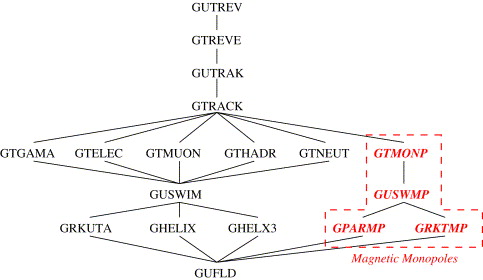
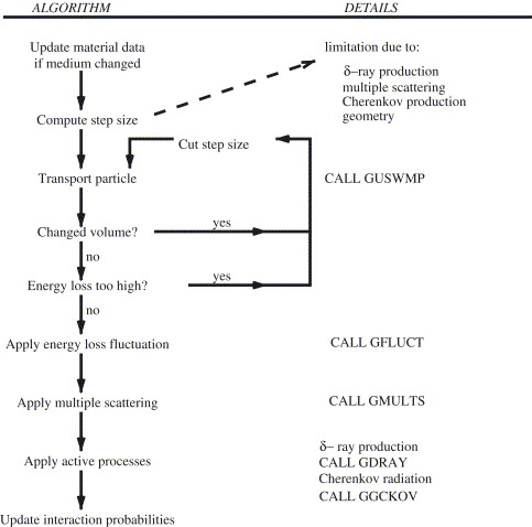
First Results
As as demonstration of principle, we present here a few Starsim event display pictures. First, we propagate 12 magnetic monopoles of varying momenta, in the STAR detector:
Now, let's take a look at a minimum bias gold-gold event that contains a pair of magnetic monopoles:
Salient features can already be seen in these graphics: large dE/dx losses and characteristic limit on the maximum radius of the recorded monopole track (this is due to the fact that the trajectory of the mm is not helix-like, but rather parabole-like). Now, lets take a look at the phi distribution of the hits, for central and peripheral gold-gold events containing monopoles:
Again, the rather intuitive feature (large peaks in phi due to a very large dE/dx produced by the monopoles) is obviously borne out in the simulation.
This is work in progress and this page is subjec to updates.
Grid-friendly Starsim production scripts
Since the production activity of STAR is migrating to, and eventually will end up running mostly in the Grid environment, this necessitates modification (which often means simplification) of the production scripts we use when running on a local or another "traditional" Unix farm facility. Here is an example of the script we have successfully used to run a Pythia simulation on the Grid (utilizing the Fermilab facility), as well as the SunGrid, with cosmetic modifications. A few things worth noting:- The bulk of the script has to do with establishing the Pythia settings which are often required in the simulations requested by the Spin PWG; the starsim proper part is located on top is is uncomplicated; it invloves dynamic loading of the necessary libraries, setting up the beam interaction diamond parameters ets
- The script needs the contents of the tarball (listed on the bottom of the page) located in its working directory; this "payload" contains the Starsim executable as well as a few shared libraries and accessory scripts necessary for its function. To be able to run on the Grid, therefore, on needs to
- Transfer the tarball and make provisions for extraction of the files
- Transfer the script below and configure it for submission with a unique serial number (any integer, really)
- The script takes only one argument, which is the serial number of the run. The rest of the run parameters are encoded in its body, which minimizes the chances of human error when submitting a large number of scripts, potentially for many different datasets
- The random number generator is seeded with the serial run number and with the Unix process ID of the script on the target machine, which for all intents and purposes guarantees the uniqueness of a sequence in each run
#!/usr/bin/ksh
echo commencing the simulation
export STAR=.
echo STAR=$STAR
#
run=$1
geom=Y2006C
ntrig=2000
diamond=60
z=120
#  >> run.$run.log 2>&1
node=`uname -n`
echo run:$run geom:$geom ntrig:$ntrig diamond:$diamond z:$z node:$node pid:$$
./starsim -w 0 -g 40 -c trace on .<<EOF
trace on
RUNG  $run     1   $$
RNDM  $$    $run
gfile o gstar.$run.fz
detp  geom $geom
vsig  0.01  $diamond
gexec  $STAR/geometry.so
gexec  $STAR/libpythia_6410.so
gexec  $STAR/bpythia.so
gclose all
gkine -1 0 0 100 -6.3  6.3 0 6.28318 -$z $z
ENER 200.0
MSEL 1
CKIN 3=4.0
CKIN 4=5.0
MSTP (51)=7
MSTP (81)=1
MSTP (82)=4
PARP (82)=2.0
PARP (83)=0.5
PARP (84)=0.4
PARP (85)=0.9
PARP (86)=0.95
PARP (89)=1800
PARP (90)=0.25
PARP (91)=1.0
PARP (67)=4.0
MDCY (102,1)=0  ! PI0 111
MDCY (106,1)=0  ! PI+ 211
MDCY (109,1)=0  ! ETA 221
MDCY (116,1)=0  ! K+ 321
MDCY (112,1)=0  ! K_SHORT 310
MDCY (105,1)=0  ! K_LONG 130
MDCY (164,1)=0  ! LAMBDA0 3122
MDCY (167,1)=0  ! SIGMA0 3212
MDCY (162,1)=0  ! SIGMA- 3112
MDCY (169,1)=0  ! SIGMA+ 3222
MDCY (172,1)=0  ! Xi- 3312
MDCY (174,1)=0  ! Xi0 3322
MDCY (176,1)=0  ! OMEGA- 3334
trig $ntrig
exit
EOF143575 2007-05-31 18:02:47 agetof
65743 2007-05-31 18:02:39 agetof.def
44591 2007-05-31 19:05:34 bpythia.so
5595692 2007-05-31 18:03:10 geometry.so
183148 2007-05-31 18:03:15 gstar.so
4170153 2007-05-31 19:05:27 libpythia_6410.so
0 2007-05-31 18:00:06 StarDb/
0 2007-05-31 18:00:59 StarDb/StMagF/
51229 2007-05-31 18:00:57 StarDb/StMagF/bfield_full_negative_2D.dat
2775652 2007-05-31 18:00:57 StarDb/StMagF/bfield_full_negative_3D.dat
51227 2007-05-31 18:00:57 StarDb/StMagF/bfield_full_positive_2D.dat
2775650 2007-05-31 18:00:58 StarDb/StMagF/bfield_full_positive_3D.dat
51227 2007-05-31 18:00:58 StarDb/StMagF/bfield_half_positive_2D.dat
2775650 2007-05-31 18:00:58 StarDb/StMagF/bfield_half_positive_3D.dat
1530566 2007-05-31 18:00:59 StarDb/StMagF/boundary_13_efield.dat
51231 2007-05-31 18:00:59 StarDb/StMagF/const_full_positive_2D.dat
1585050 2007-05-31 18:00:59 StarDb/StMagF/endcap_efield.dat
1530393 2007-05-31 18:00:59 StarDb/StMagF/membrane_efield.dat
15663993 2007-05-31 18:03:31 starsim
36600 2007-05-31 18:03:37 starsim.bank
1848 2007-05-31 18:03:42 starsim.logon.kumac
21551 2007-05-31 18:03:48 starsim.makefileProduction overview
As of spring of 2007, the Monte Carlo production is being run on three different platforms:
-
the rcas farm
-
Open Science Grid
-
SunGrid
Miscellaneous scripts
aVMC
VMC C++ Classes
StarVMC/StarVMCApplication:
- StMCHitDescriptor
- StarMCHits
- Step
- StarMCSimplePrimaryGenerator
Example of setting the input file: StBFChain::ProcessLine ((StVMCMaker *) 0xaeab6f0)->SetInputFile("/star/simu/simu/gstardata/evgenRoot/evgen.3.root");
In general, StBFChain sets various attributes of the makers.
New chain options must be added in BigFullChain.h