Getting a publishable dNdeta distribution with the EPD
Updated on Sun, 2020-04-12 21:31. Originally created by lisa on 2020-04-07 10:46.
This page has some useful information, but it was never really finished so the message is never really concluded.
On this page, I introduced the STAR EPD Fast Simulator.
On this page, I showed how dN/deta, inputted into the Fast Simulator could be hand-tweaked to reproduce the dN/dnMIP distributions in the 16 rings to an excellent degree.
To get a publishable result, we have to go beyond hand-tweaking, though. On this page, I go through some attempts.
Following the PHOBOS example, I have 18 bins in eta, and thus 18 dN/deta values that I can treat as "parameters" to vary to fit the data. On this page, I varied them by hand, and things looked quite promising. However.... when I give the problem to Minuit, it fails. It is a 18-parameter fit, but honestly that's not so bad (speaking as an HBT guy). The number of degrees of freedom are 16 times the number of bins in the nMIP distribution, which is typically 40 at least (binning of 0.1 nMNIP), so say 600 degrees of freedom. Again, not outrageous, speaking as an HBT guy.
So... what's the problem? Two problems: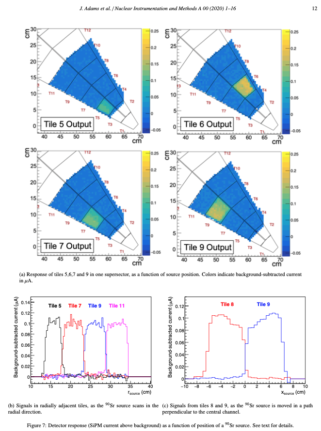
Figure 1 - Figure 7 from the EPD NIM article, showing the results of an x-y scan over the position of ionization in a supersector. See the article for details.
In retrospect, both of these problems could have been expected.
First of all, sorry for the naming convention here. In EPD parlance, "nMIP" is basically "gain-calibrated ADC value." It is a continuous variable, and the calibration is such that "nMIP=1" is at the MPV (most probable value) of the single-MIP distribution. ("MIP" = minimally ionizing particle.) So, a tile can easily have nMIP=1.5 in some event.
I now want to define "#MIP" which is really the number of MIPs that pass through a tile in a given event. Two differences from nMIP
Why might this be better than Method 1? Well, it removes (1) the randomness of the Landau fluctuations and (2) fine details like the non-uniformity of response at the cm-scale. Both of these things were simply "distracting details" that can only hurt the fit convergence, not providing extra information.
The following two sets of plots should indicate how well we can determine the fraction of 1-,2-3-,n-hit events, for each ring:
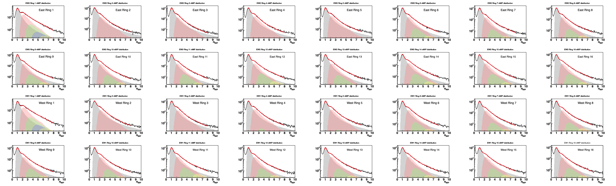
Figure 2 - STAR measurements of nMIP (calibrated ADC) distributions from 10-40% Au+Au collisions at 27 GeV, meassured in 2019. All 12 tiles of Ring 1 contribute to the Ring 1 plot, while all 24 tiles of ring M contribute to the Ring M plot. East and West rings are plotted separately. Black histogram=data. Red line=Multi-MIP fit to the data. Shaded regions = contributions from one (grey), two (red), three (green), four (blue) and five (yellow) hit events are shown. These sum to make the red line.
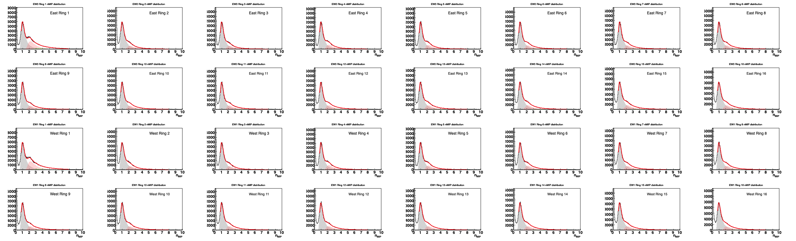
Figure 3 - Same as figure 2, but on a linear scale.
The above plots show that the distributions can be quite well fit in terms of single- and multiple-hit events, and we can extract the fraction of such events. The EPD FastSim can also predict these fractions, given a dN/deta distribution. As someone who has done literally tens of thousands of these plots, I can tell you that once the fraction gets at the percent level (so, like 3+ hits in the outer rings), the contribution is so small that the fit can pick up fluctuations.
Below, see the fraction of 1-, 2-, 3-,... hit events in the 16 rings of the EPD (east and west are averaged here).
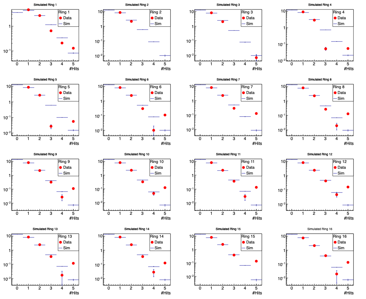
Figure 4: Red points show the distributions of 1-hit, 2-hit, 3-hit, etc events, as determined by the fits shown in figures 2 and 3. Histogram shows these distributions as determined by the FastSimulator. Note that these latter numbers do not come from fits to energy loss spectra, but directly from knowing the number of particles that pass through a tile in a given event. Integral of these distributions equals the number of tiles in the ring-- 12 for ring 1 and 24 for rings 2-16. Note that we do not calculate the fraction of zero-hit events for the data, but they are constrained by the integral. I.e. it is trivial.
.png)
Figure 5: Same as figure 4, but on a linear scale.
The data are compared to simulated calculations in figures 4 and 5 above. The agreement isn't bad (again I repeat that 3+ hit contributions are (1) small and (2) can be unstable in the outer rings). So, I tried to use the 18 eta bins as parameters, and tell Minuit to vary those parameters to make the calculations match the data. Nice idea, but once again, even though the Landau fluctuations are not contributing, the other fluctuations mean that even for THE SAME DISTRIBUTION DN/DETA, the chi2 can vary up to 5%, and that drives Minuit bonkers. The fit cannot progress.
Why are we even doing simulation, actually? For every event, each of our tiles reports an nMIP value, between 0 and 20. (Actually, we have a threshold ~0.3 to get rid of the noise, but still, there shouldn't be much "real" signal below there, as seen in the fits of figures 2 and 3.) How about just fill a histogram with tile.nMIP() as the weight?
Well, that's likely to be a pretty bad idea, since the Landau fluctuations can be gargantuan. We found that the best event-plane resolution and the best centrality resolution was obtained when using truncated nMIP values (i.e. if nMIP is below threshold, set it to zero, and if nMIP is above MAX, set it to MAX. MAX ~ 2.0 seems best). That's fine for event plane resolutions, but if we start imposing truncations to get yields, that's a pretty obvious correlation and rather arbitrary.
So, if we follow that route in the data.... we will get a distribution. Yay? But how do we know whether to trust it? Answer: use the EPD FastSim.
Sorry, this discussion got cut short due to movements in other directions...
Summary:
This page has some useful information, but it was never really finished so the message is never really concluded.
On this page, I introduced the STAR EPD Fast Simulator.
On this page, I showed how dN/deta, inputted into the Fast Simulator could be hand-tweaked to reproduce the dN/dnMIP distributions in the 16 rings to an excellent degree.
To get a publishable result, we have to go beyond hand-tweaking, though. On this page, I go through some attempts.
- Treat the 18 eta bins as input parameters to the EpdFastSim, which then produces dN/dnMIP for the 16 rings. Perform a chi2 fit to these dN/dnMIP spectra.
- Fail. Fit does not converge. Not surprising, in retrospect.
- With Multi-Landau fits, extract dN/d#MIP distributions from the 16 rings. And then use the 18 eta bins as input parameters to the EpdFastSim, which then produces dN/d#MIP for the 16 rings. Perform a chi2 fit to these dN/d#MIP spectra.
- Fail. Fit does not converge. Computation time requirement way too high.
- Turn to the data itself. Make a "nMIP-weighted dN/deta"
- For each EPD tile TT in an event:
- TVector3 p = StEpdGeom::RandomPointOnTile(TT.id()) - PrimaryVertex;
- dNdetaData->Fill(p.Eta(),TT.nMIP());
- Simulator says it will fail. Not surprising. Very big Landau fluctuations.
- For each EPD tile TT in an event:
- Turn to the data itself and treat the EPD as a "hit detector".
- For each EPD tile TT in an event:
- if TT.nMIP() > thresh, dNdetaData->Fill(p.Eta());
- then, find the correction using EpdFastSim.
- Should work if multiple-hit probability isn't huge.
- For each EPD tile TT in an event:
Method 1 - fitting dN/dnMIP
Following the PHOBOS example, I have 18 bins in eta, and thus 18 dN/deta values that I can treat as "parameters" to vary to fit the data. On this page, I varied them by hand, and things looked quite promising. However.... when I give the problem to Minuit, it fails. It is a 18-parameter fit, but honestly that's not so bad (speaking as an HBT guy). The number of degrees of freedom are 16 times the number of bins in the nMIP distribution, which is typically 40 at least (binning of 0.1 nMNIP), so say 600 degrees of freedom. Again, not outrageous, speaking as an HBT guy.
So... what's the problem? Two problems:
- Probably the biggest one. The "theory" curve comes from a Monte-Carlo-sampled (Poisson fluctuations on the number coming from any eta bin, then uniformly (if v1=v2=0) randomly distributed in z), from a random-sampling from the Vz distribution, then random Landau energy loss in the tiles, to produce the nMIP spectra. Which is fine..... except..... Minuit requires that a fixed set of input parameters makes exactly the same chi2 (or whatever is being minimized), and this random business just won't do that. It drives the minimizer crazy and it won't converge. Generating 50,000 events per iteration gives chi2 fluctuations on the order of 5%, even when having THE SAME VALUES of dN/deta. This is out of reach.
- Also.... the dN/dnMIP distributions look pretty good! (Again see here.) But.... hey they are not perfect. Why would they be? The simulator assumes every particle is a MIP and all particles pass through the material at the same angle, and the response of the tile is uniform across its face. These are not horrendous assumptions, but with so many degrees of freedom, you really do want to have the "right" theory. E.g. here is figure 7 from the EPD NIM paper (arxiv.org/abs/1912.05243) where there is clearly a ~20% variation in "gain" across the face of the typical tile:
Figure 1 - Figure 7 from the EPD NIM article, showing the results of an x-y scan over the position of ionization in a supersector. See the article for details.
In retrospect, both of these problems could have been expected.
Method 2 - Fitting dN/d#MIP
First of all, sorry for the naming convention here. In EPD parlance, "nMIP" is basically "gain-calibrated ADC value." It is a continuous variable, and the calibration is such that "nMIP=1" is at the MPV (most probable value) of the single-MIP distribution. ("MIP" = minimally ionizing particle.) So, a tile can easily have nMIP=1.5 in some event.
I now want to define "#MIP" which is really the number of MIPs that pass through a tile in a given event. Two differences from nMIP
- It is an integer value, unlike nMIP which is a continuous value.
- Whereas a tile has a well-defined nMIP value for every event, #MIP cannot be determined event-by-event. Rather, one takes the nMIP distribution and does a multi-MIP fit, to extract the fraction of times 0, 1, 2, 3, 4... MIPs passed through the tiles, on a statistical basis.
- measure the dN/nMIP spectra for the 16 rings (just like in Method 1)
- fit the dN/nMIP spectra to extract dN/d#MIP distributions for the 16 rings (see here for just one maybe 50 pages discussing this)
- give Minuit the 18 values of dN/deta as parameters, and demand that it produce (again, through EpdFastSim) the same dN/d#MIP spectra as in the data.
Why might this be better than Method 1? Well, it removes (1) the randomness of the Landau fluctuations and (2) fine details like the non-uniformity of response at the cm-scale. Both of these things were simply "distracting details" that can only hurt the fit convergence, not providing extra information.
The following two sets of plots should indicate how well we can determine the fraction of 1-,2-3-,n-hit events, for each ring:
Figure 2 - STAR measurements of nMIP (calibrated ADC) distributions from 10-40% Au+Au collisions at 27 GeV, meassured in 2019. All 12 tiles of Ring 1 contribute to the Ring 1 plot, while all 24 tiles of ring M contribute to the Ring M plot. East and West rings are plotted separately. Black histogram=data. Red line=Multi-MIP fit to the data. Shaded regions = contributions from one (grey), two (red), three (green), four (blue) and five (yellow) hit events are shown. These sum to make the red line.
Figure 3 - Same as figure 2, but on a linear scale.
The above plots show that the distributions can be quite well fit in terms of single- and multiple-hit events, and we can extract the fraction of such events. The EPD FastSim can also predict these fractions, given a dN/deta distribution. As someone who has done literally tens of thousands of these plots, I can tell you that once the fraction gets at the percent level (so, like 3+ hits in the outer rings), the contribution is so small that the fit can pick up fluctuations.
Below, see the fraction of 1-, 2-, 3-,... hit events in the 16 rings of the EPD (east and west are averaged here).
Figure 4: Red points show the distributions of 1-hit, 2-hit, 3-hit, etc events, as determined by the fits shown in figures 2 and 3. Histogram shows these distributions as determined by the FastSimulator. Note that these latter numbers do not come from fits to energy loss spectra, but directly from knowing the number of particles that pass through a tile in a given event. Integral of these distributions equals the number of tiles in the ring-- 12 for ring 1 and 24 for rings 2-16. Note that we do not calculate the fraction of zero-hit events for the data, but they are constrained by the integral. I.e. it is trivial.
Figure 5: Same as figure 4, but on a linear scale.
The data are compared to simulated calculations in figures 4 and 5 above. The agreement isn't bad (again I repeat that 3+ hit contributions are (1) small and (2) can be unstable in the outer rings). So, I tried to use the 18 eta bins as parameters, and tell Minuit to vary those parameters to make the calculations match the data. Nice idea, but once again, even though the Landau fluctuations are not contributing, the other fluctuations mean that even for THE SAME DISTRIBUTION DN/DETA, the chi2 can vary up to 5%, and that drives Minuit bonkers. The fit cannot progress.
Method 3 - Just use the data and the nMIP from each event!
Why are we even doing simulation, actually? For every event, each of our tiles reports an nMIP value, between 0 and 20. (Actually, we have a threshold ~0.3 to get rid of the noise, but still, there shouldn't be much "real" signal below there, as seen in the fits of figures 2 and 3.) How about just fill a histogram with tile.nMIP() as the weight?
Well, that's likely to be a pretty bad idea, since the Landau fluctuations can be gargantuan. We found that the best event-plane resolution and the best centrality resolution was obtained when using truncated nMIP values (i.e. if nMIP is below threshold, set it to zero, and if nMIP is above MAX, set it to MAX. MAX ~ 2.0 seems best). That's fine for event plane resolutions, but if we start imposing truncations to get yields, that's a pretty obvious correlation and rather arbitrary.
So, if we follow that route in the data.... we will get a distribution. Yay? But how do we know whether to trust it? Answer: use the EPD FastSim.
Sorry, this discussion got cut short due to movements in other directions...
»
- lisa's blog
- Login or register to post comments