Extracting dN_ch/dη from EPD data

Results in this blogpost are based on a HIJING+GEANT simulation of 5000 |Vz|<5 cm events with b = 7...8 fm (roughly ~16M primary tracks), with settings starver:SL19e, geom:y2018a. The list of simulated MuDST files used in this analysis is given in /star/u/mcsanad/work/epd/sim2020/roland/SL19e_geom18a_b78_Vz5_5kevt.mudst.list

These previous blogposts dealt with extracting dN/dη from EPD data via unfolding:

• Unfolding EPD data with various response matrices - May 18., 2020
• What particles cause hits in the EPD? - May 13., 2020
• Testing the unfolding procedure with various input dN/deta distributions - May 5., 2020
• Unfolding dN/deta with RooUnfold - May 1., 2020

Since the EPD is mainly capable of detecting charged particles, let us see how it does in extracting dN_ch/dη instead.

Primary charged track ratios

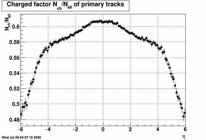
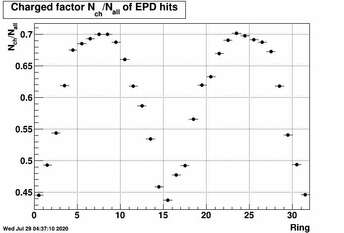
In the simulations, we can check how many primary particles are charged and how many primary particles are neutral, as well as how many EPD hits are caused by charged and neutral primary tracks (this of course requires tracking back any given EPD hit to the original primary track that caused it through its daughters). Here are the corresponding N_ch(η)/N_tot(η) and N_ch(ring)/N_tot(ring) plots:

FIG. 1: Nch(η)/Ntot(η) ratio of primary tracks from HIJING	FIG. 2: Nch(ring)/Ntot(ring) primary track ratio of EPD hits from HIJING+GEANT

Remark: one may be surprised why the charged fraction vs pseudorapidity is not on average 2/3, as one would expect based on simple hadron counting. The reason for that is (see this blogpost for details):
(i) 4% of all HIJING primary tracks are gammas (for which there are no neutral counterparts);
(ii) there are somewhat more neutral than the half of charged pions - given in percentage of all primary tracks: 27% π⁰, 23% π^-, 23% π⁺.
Hence on average, only ~57% of all primary tracks are charged.

Methods of extracting dN_ch/dη

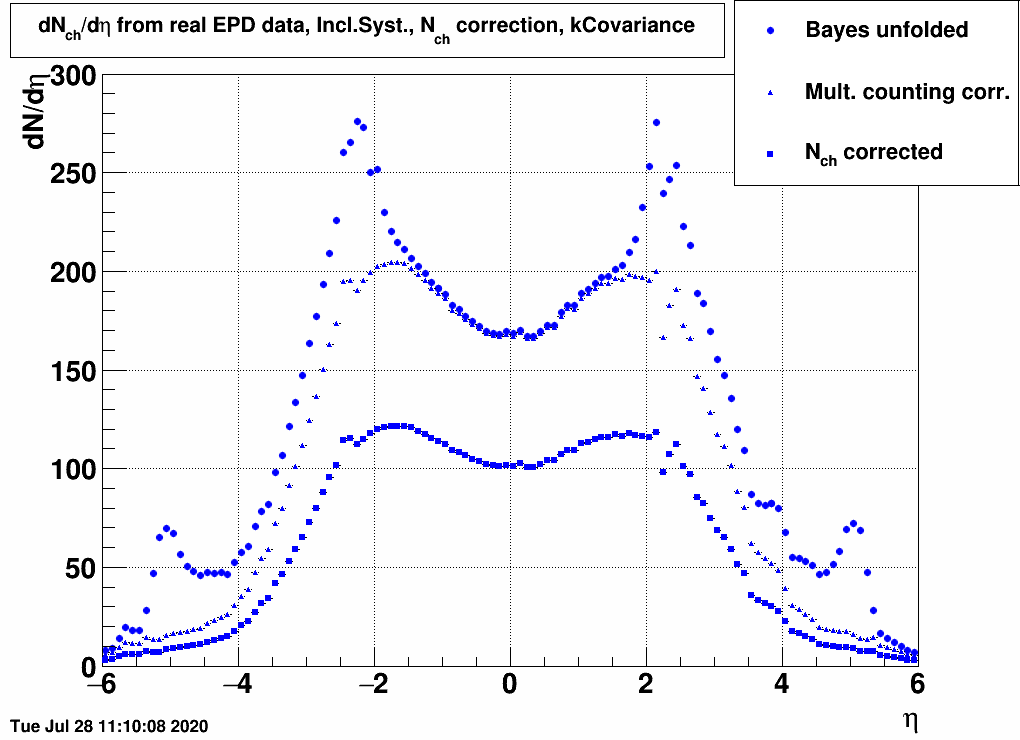
There are three possible methods to extract dN_ch/dη from the EPD data (which of course does not know about the charge of the particles causing the hits):

1. Unfolding dN/dη and then correcting via N_ch(η)/N_tot(η) determined from simulations (Fig. 3)
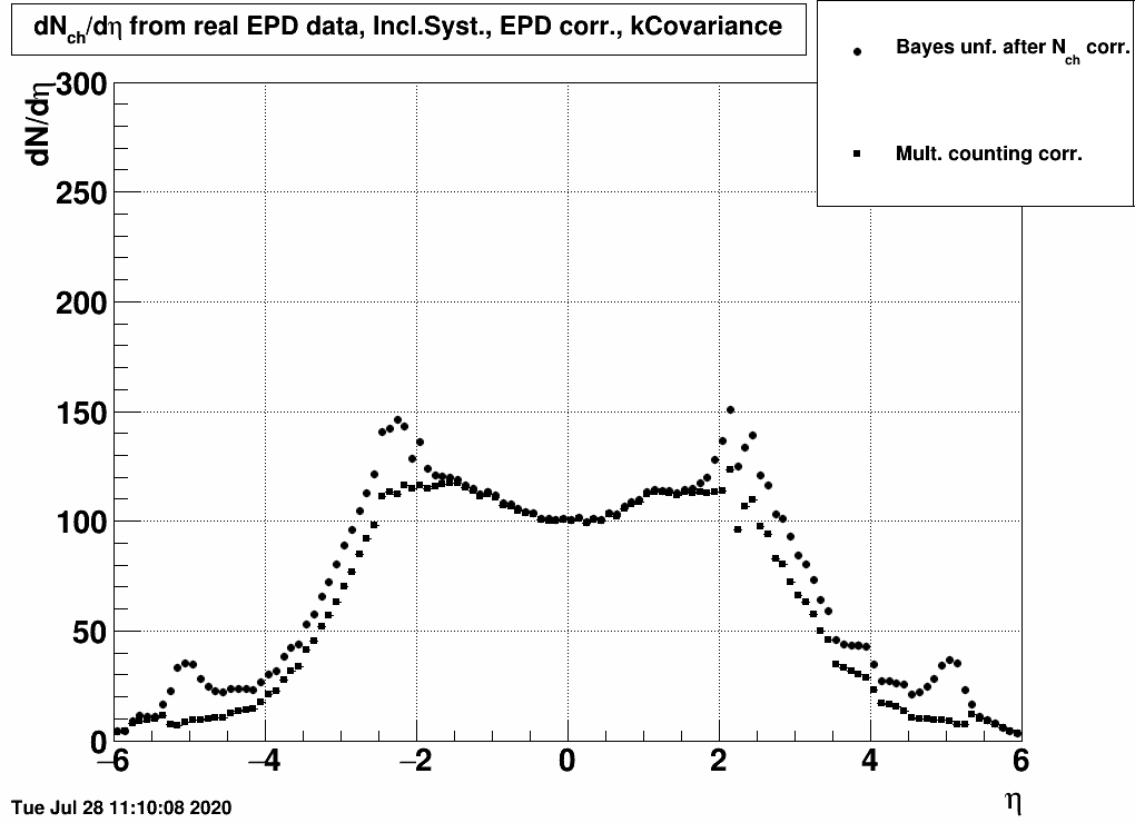
2. Correcting the ring-by-ring EPD distribution via N_ch(ring)/N_tot(ring), and then unfolding this "corrected" EPD distribution (Fig. 4)
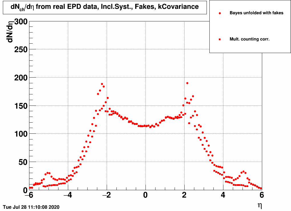
3. Using the built-in "Fakes" method of RooUnfold (where neutral particles then are meant to cause "fake" hits), which is supposed to handle exactly this (Fig. 5)
   

Here are these three methods applied to 19.6 GeV STAR data (note that there is a "multiple counting correction" applied in each case, see details in the next subsection, as well as at the end of an earlier blogpost):

FIG. 3: Correcting by Nch(η)/Ntot(η)	FIG. 4: Correcting by Nch(ring)/Ntot(ring)	FIG. 5: Correcting via RooUnfold's fakes

Note that the measured data has a different Vz distribution, which should be reproduced by the simulations, but they are not yet (for simplicity).

Multiple counting correction

Recall that an appropriate "efficiency correction" was applied to correct for "multiple counting", i.e. taking care of the fact that one primary track can create multiple hits. This correction factor is defined for each η bin as

   ε = Σ_i[F_i×N_i + (1-F_i)] / N_prim.tracks

where i runs through all primary tracks, N_i is the number of EPD hits the given track caused, and F_i = 1 if N_i>0 and 0 otherwise. The reason for this is that RooUnfold puts an entry into the to-be-reconstructed distribution of each hit, as well as for each "miss", i.e. primary track without a hit. This information is used to do the reconstruction taking into account "misses". Note that hence ε>1 always (each primary track contributes by at least 1 to the numerator).

One can create such an "efficiency" based on charged or all (charged+neutral) primary tracks, and Fig. 6. below shows how they look like in the simulation applied in the calculations of this blogpost.

FIG. 6: Multiple counting corrections for all & charged tracks

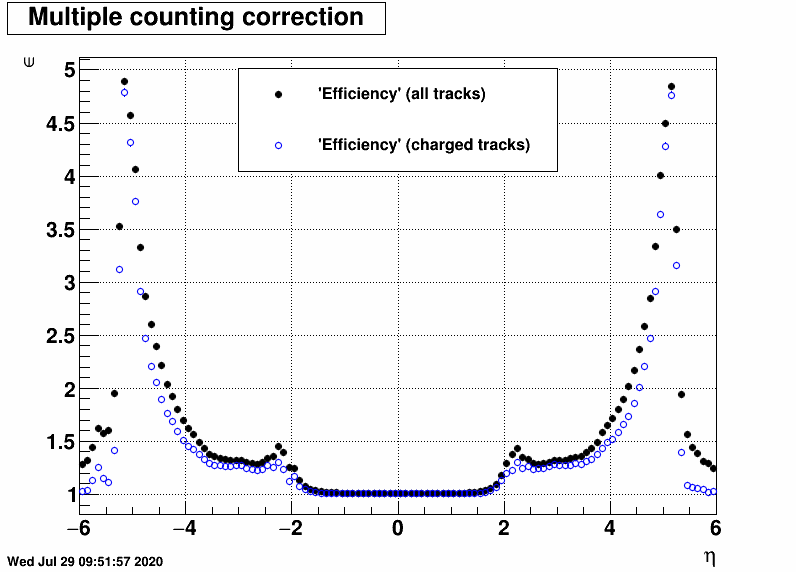Clearly one has to use the appropriate one when correcting for this multiple counting. However, in the first case (Fig. 3) it is not entirely clear which one to use: if one corrects for this before multiplying by the charged factor of Fig. 1, then using EfficiencyAll is more logical. However, if one would correct for the multiple counting after multiplying by the charged factor, then using EfficiencyCharged would be more logical. But these two yield a somewhat different result. Here I used EfficiencyAll, and then multiplied by the charged factor.

Results on dN_ch/dη via the three methods

Here are the final results from the three methods compared:

FIG. 7: Three methods of extracting dNch/dη from 19.6 GeV EPD data

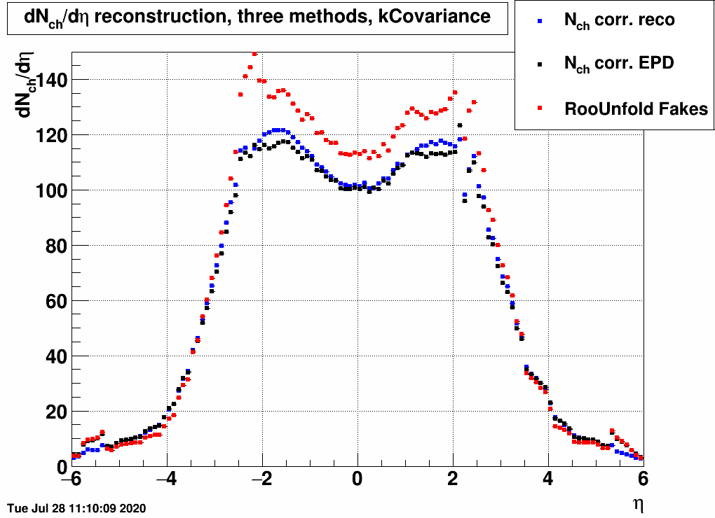Apparently these methods yield approximately the same result in the EPD region (2<|η|<5), c.f. unfolding simulation dependent uncertainty detailed in
drupal.star.bnl.gov/STAR/blog/mcsanad/unfolding-epd-data-various-response-matrices
where it is seen that the simulated dataset's pseudorapidity distribution creates a ~10% uncertainty in dN/dη, this uncertainty is apparently comparable to the one related to moving from dN/dη to dN_ch/dη visible above.

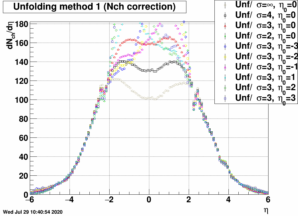
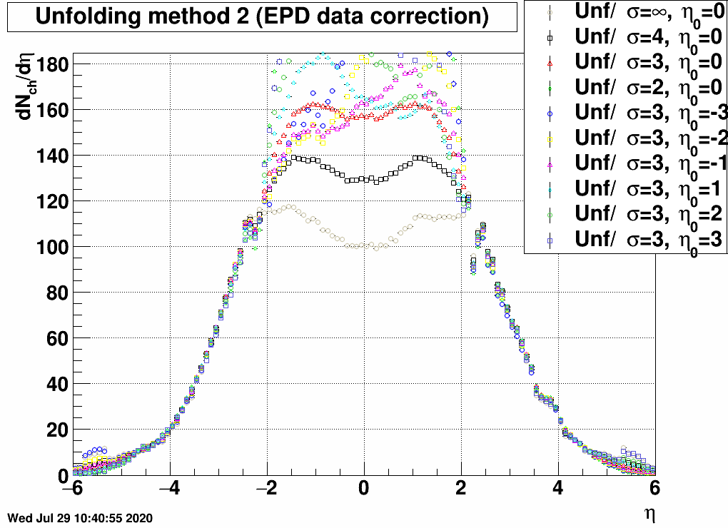
Simulation uncertainty of reconstructed dN_ch/dη

Now the error related to the simulation details (in particular the pseudorapidity distribution) can be checked similarly to the above mentioned previous blogpost:

FIG. 9: Unfolding uncertainty method 1 (correcting by Nch(η)/Ntot(η))	FIG. 10: Unfolding uncertainty method 1 (correcting by by Nch(ring)/Ntot(ring))	FIG. 11: Unfolding uncertainty method 1 (correcting via RooUnfold's fakes)

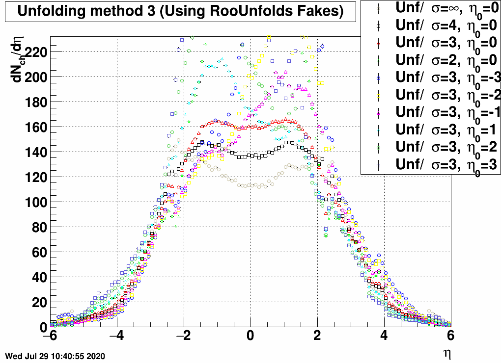Again the uncertainty is small when being in the EPD range (2<|η|<5) for the first two cases, but larger when using the Fake() method of RooUnfold. Fakes in principle does the following:

• Register each fake hit (in our case, hit with a neutral primary cause), in EPD ring bins.
• Add an extra bin to the list of causes (i.e. an extra truth bin corresponding to fake causes), the value of this shall be the total number of fakes.
• Add an extra row to the response matrix (at the extra eta bin, for each ring bin), with value of the number of fakes at given ring bin.
• Reconstruction (unfolding) with these extra bins.
• Remove extra bins after unfolding.

This should in principle mean that the unfolded result (dN/deta) first contains an extra bin with the estimated number of fakes (fake causes), which is then removed. Probably this is less sophisticated as compared to us also knowing the η value of the "fake" hit. However, correcting by N_ch(ring)/N_tot(ring) before unfolding and correcting by N_ch(η)/N_tot(η) after unfolding yields the same result, so I'm not sure why using fakes yields a different result, which is so dependent on the simulations η distribution.