This is a continuation of: drupal.star.bnl.gov/STAR/blog/rjreed/centrality-epd-take-3 and drupal.star.bnl.gov/STAR/blog/rjreed/epd-and-weighted-average

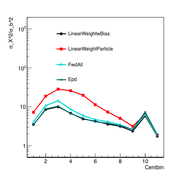
I have been spending some time trying to understand this plot:

Figure 1: Resolution as defined by the sigma of a particular observable squared, over the sigma of the impact parameter squared, for a given centrality bin.  The centrality bins are 0,5,10,20,30,40,50,60,70,80,90,100, and in this plot the most central is on the right.  The discontinuity we see going from the most central two bins to the others is due to change in bin size.

The linear weight was developed by Mike at: drupal.star.bnl.gov/STAR/blog/lisa/ring-weights-estimating-global-quantities-linear-sums

I have verified that the math and code make sense.  In Figure 1, EPD is the Nmip sum (with a Nmip max of 2), forward all is simple counting all the charged particles in the EPD acceptance, Linear weight is using the NMip distribution ring by ring, and Linear Weight Particle divides the particles into rings but does not put any detector effects in.

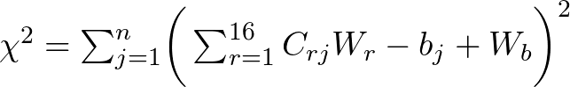
The linear weight method that Mike develops minimizes the squared residual -

where we use b as the global quantity Gj.  Surprisingly, this method did not yield better results than the simple counting methods.  The weights that popped out are:
Repeating the weights:
ring      weight
    1    0.273525
    2    0.0296001
    3    -0.0601397
    4    -0.0477917
    5    -0.0337742
    6    -0.0232543
    7    -0.0117203
    8    -0.00703337
    9    -0.0024524
    10    0.00399249
    11    0.00605742
    12    0.00908568
    13    0.00985799
    14    0.0102809
    15    0.013745
    16    0.0136804

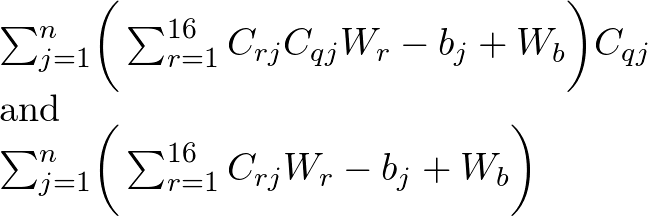
I noticed two things about this distribution, one is that the first ring has a weight an order of magnitude higher than all the rest, and that the sign changes back and forth as one goes down.  The problem is that ring 1 is correlated with b (at this energy), rings 3 - 16 are anti-correlated.  My expectation would be that a proper weighting would then have the weights of opposite signs.  I also thing the large weight of ring 1 is due to the much larger amplitude of the signal in this ring.  But this then "double counts" the signal when the observable is calculated:

Based on this thought, I decided to look at a different methodology, where I looked at the Pearson Correlation Coefficient (PCC) ring by ring, which is a measure of the linear correlation between X and Y.  Mathematically this is defined as:

This is the covariance divided by the standard deviation of each distribution.  For the weights, I arbitrarily chose them to be the PCC for each distribution, which gave:

Ring 1 correlation factor 0.896573
Ring 2 correlation factor 0.0672031
Ring 3 correlation factor -0.824721
Ring 4 correlation factor -0.876886
Ring 5 correlation factor -0.903983
Ring 6 correlation factor -0.914713
Ring 7 correlation factor -0.914244
Ring 8 correlation factor -0.925129
Ring 9 correlation factor -0.924578
Ring 10 correlation factor -0.920478
Ring 11 correlation factor -0.925422
Ring 12 correlation factor -0.917096
Ring 13 correlation factor -0.920544
Ring 14 correlation factor -0.924014
Ring 15 correlation factor -0.910315
Ring 16 correlation factor -0.912998

As I had suspected should be the case.  This gave the result:

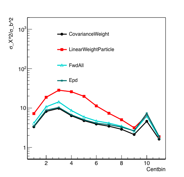
Figure 2: A repeat of Figure 1, but with the PCC method (covariance weight) substituted instead.  This does as well as the EPD method in peripheral bins, and a bit better in the central bins.

Mike's valid criticism here is that I didn't minimize anything, simply asserted something to be true.  The reason I think this works out is that to determine the centrality, we take the distribution in question and slice it up into quantiles.  With this method, minimizing the difference between the distribution and b is not the goal, rather we would want to increase the correlation of our distribution with b so that our determination of centrality bins by quantiles gives the best result.  By using weights that are of similar values (other than for ring 2 which has little correlation with b), each ring has an equal "chance" to contribute, with the only weighting being the signal itself. 

These distributions are not linearly correlated, so it may be that there is a better weighting methodology based on a different assumption, however this naturally increases the correlation with b, though admittedly not minimizing the distance.  I attempted to include these weights in the minimization routine, but this yielded much worse results (and similar weights as before).

To further check on the linear minimization routine, I looked at what happened if I only considered the first ring:
     ring      weight
    1    0.258207

The result is very close to the original weight.

For two rings:
 ring      weight
    1    0.294981
    2    -0.0810424

And for three:
     ring      weight
    1    0.276169
    2    0.0157972
    3    -0.122849

The distribution is thus dominated by the first ring - and the weight is what one would expect if minimizing just the difference of the first ring with the second.  (I did not try to see what happens if we neglect the first ring.)

If we look at the rings separately:

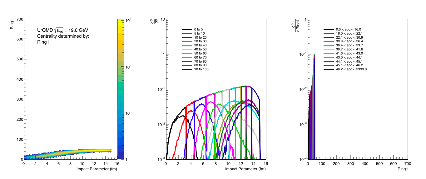
Figure 3: Analysis of ring 1 Nmip distribution, essentially if we used only the first ring for centrality distribution.

Figure 4: Analysis of ring 2 Nmip distibution.  We see here that it really doesn't correlate well with b.

Then, if we add these two with their linear weights, we find:

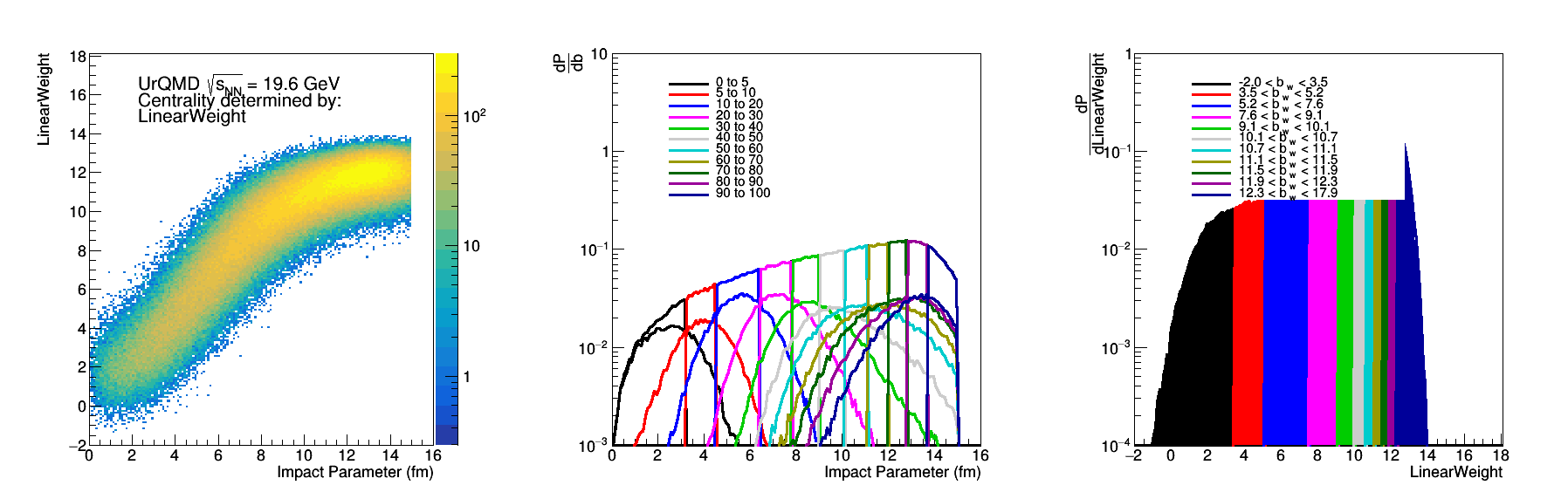
Figure 5: Analysis of adding ring 1 and 2 together using the linear weights.  It is slightly worse than ring 1 alone (which I think is not surprising giving the structure of ring 2).

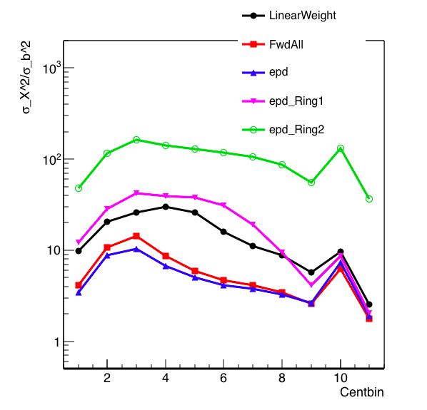
Figure 6: The resolution plot with ring 1 and two included.  I still need to add the ring1+ring2 distribution.  (I might take this out to ring 3 and do the same exercise with the covariance .. not mathematically rigorous but I see the distributions taking shape).

All this being said - it should be possible to minimize a distribution wrt b and have the resolution do better.  I had thought that including sigma could help - this would bring the result closer to the PCC method that seems to be performing well.  This I thought would decrease the dependency on ring 1 alone.

Taking the derivative with respect to weight and setting it equal to zero, you get:

Unfortunately the results were the same ... and when I looked at the standard deviation, it was similar from ring to ring, even though the mean value was different.

I tried again with putting the expected value (b) in the denominator, which also failed but at this point I'm not convinced that it wasn't a coding error so I can try again.

Mike has also suggested putting an offset in, which would turn this into a 17 linear equation problem.  I will define the residual as:

Then the derivative is with respect to both Wr and Wb...  This gives us 17 equations of the form:

We can write these in the same form that Mike did (A_{q,r}W_r = B_q.

If, for a moment, we only had 2 rings so that I can write this more simply (and I drop for the moment the summation over all events - it's there of course), this would look like:

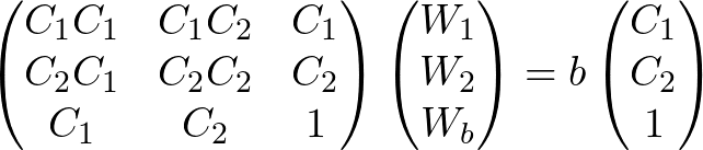
Basically, the bias forms the 17th row.  Adding this into the code, I find:
  1    0.00680961
    2    -0.01347
    3    -0.0332635
    4    -0.0302532
    5    -0.0268818
    6    -0.0247482
    7    -0.0237771
    8    -0.0243792
    9    -0.0245445
    10    -0.0240506
    11    -0.0242869
    12    -0.0250776
    13    -0.0246544
    14    -0.0259138
    15    -0.0249609
    16    -0.026065
    17    13.319

Yup... that seems to be it.