JANs sub-page for FGT ops

 JAN: this page was created after Jerome opened write privileges

RENEE : I am writing on Jan's child page

Renee's Child Page

Is it this easy to have a child?

at the beginningyes, with time it gets more serious responsibility, but parents mature in sync (or not), Jan

Existing Framework For FGT Simulations

With the completion of the FGT hardware review, focus must now be made on the creation and implementation of efficient analysis algorithms. To this end a framework for creating simulation files must be established. Here I document the existing framework I created this past summer for a small FGT project.
    The creation of simulation files within STAR is handled in two steps.

• starsim is called with a PYTHIA kumac, creating a fzd file.
• The fzd file is converted to a full muDst with the bfc.

The kumac sets all parameters of the underlying physics events, while the bfc handles the fine tuning of the reconstruction of the STAR detector.
    In the following analysis the simulation was split by the underlying physics processes: those producing W bosons and those from QCD 2->2 interactions. Both are produced with the geometry UPGR13 and sqrt(s) = 500 GeV, in accordance with the FGT upgrade. Moreover, each kumac accepts a random number seed to ensure that different jobs are independent of each other.  Specific details are included below,

Detailed log files can be found at

while the existing files are at

Attached are the relevant scripts (the _.txt has been added to get around DRUPAL attachment restrictions), although the hardcoded paths are no longer valid.  The master script is submit_simulations.csh, which submits all the others to the RCAS queue star_cas_big.  In particular, W_job.csh and hadron_job.csh are each called with the command line arguments

The *_job.csh scrips then call the starsim and bfc with the necessary arguments passed as appropriate.

Filtered Simulations For The Development of Electron/Hadron Discrimination Algorithms

Critical to the upcoming flavor physics at STAR is efficient electron identification in the endcap, particularly amongst the dominant charged hadron/meson background.  The development of such discrimination algorithms, however, requires extensive simulations.  To reduce the computational burden of these simulations to a practical level we must modify starsim, reconstructing only those events of interest.

In this case we require electrons and charged hadrons/mesons in the endcap, and by adding a filter to PYTHIA we can ensure that only events matching the this criteria are reconstructed.  Below is a small study showing the significant reduction in computing time gained with this filtering.

The filtered simulations required a charged hadron or meson in the endcap with p_T > 15 GeV before GSTAR was allowed to reconstruct the event.  Candidate refers to an event meeting the above requirements in the PYTHIA record, and projected refers to an extrapolation estimate for 80 pb^-1.

Looking at the tracks in the GEANT record we see that the filtering worked as described.  Here every charged hadron/meson in every reconstructed event is shown, and in the Filtered sample we see a sharp cutoff at 15 GeV exactly as expected. 

The same analysis can be done for the W boson simulations, here instead requiring an electron(positron) from a W decay in the endcap with p_T > 15 GeV.

Again, comparing the two files shows the desired effects

In both cases the computational demands seem impractical, but one has to remember that this extrapolation is based on the use of a single processor.  Real jobs will be run in parallel, significantly reducing the projected times to more reasonable levels.  Despite the reduction, however, it might still be necessary to reduce the desired integrated luminousity slightly.

Filtering PYTHIA Events In Starsim

Within the STAR framework, simulation files are created with the command starsim which runs both PYTHIA and GEANT.  Unfortunately, this means that there is no straightforward way to filter PYTHIA events before the GEANT reconstruction and producing simulation files for rare events can be very time consuming, as most of the CPU is wasted on the GEANT reconstruction of undesired events.

The trick around this is to modify the PYTHIA libraries themselves.  In particular we want to modify the PYEVNT subroutine which is run during the generation of each PYTHIA event.  Begin by

•     Checking out a copy of the pythia libraries from cvs
•     Create a back up of pyevnt.F in case anything goes wrong
•     Open up pyevnt.F in your favorite text editor
•     Rename SUBROUTINE PYEVNT to SUBROUTINE PYEVNT_ORG
•     Now create your own subroutine, SUBROUTINE PYEVNT
•     Copy the variable declarations and commonblocks from the original PYEVNT

The body of this new subroutine will in general go as the following

Note that to avoid too many nested if loops we abort when the first test fails.

For example, consider an analysis requiring a high energy electron in the endcap.  The usual PYTHIA settings allow one to require a high energy electron, but there is no way to restrict its location in the detector.  So in the above pseudocode becomes

The main background to the above is charged hadrons/mesons.  In order to filter these we require that the particle has a charge of +/- 1, that is has the PDG ID of a hadron or a meson, that it has not decayed in the PYTHIA record, and fulfills the kinematic requirements.

Once pyevnt.F has been succussfully modified it must be compiled with cons, and the path to the compiled library itself must be explicitly set in the kumac.  For example,

must be replaced by

Examples of modified pyevnt.F files for both the electron example and the jet example are attached, as is a kumac for use with the jet example.

List of available M-C event samples (Jan)

.

M-C Event Samples Available   

1. General  setup, assumptions
   1. use UPGR13 geometry
   2. run in SL07e
   3. use PPV vertex finder in reco
   4. displace & smear vertex in GEANT in X-Y plane: x0=+1mm, sig=200us, y0=-2mm, sig=200um (except setA)
   5. beam energy sqrt(s)=500 GeV
   6. detectors passed by track thrown at various eta at 3 Z-vertex location of -60, -30 an 0 cm.
      

---

---

2. setA (produced by Mike @ MIT)

BFC w/ generic vertex finder has ~50% efficiency,

Vertex distribution: Gauss(Z=0, sigZ=60cm, Z=Y=0, sigX=sigY=0)

Type of events	total events	time per event
Pythia, minB	400K, 100 jobs	GSTAR: 8.4 sec, BFC ???

Files location: 80K eve at IUCF disk: /star/institutions/iucf/kocolosk/2008-02-15-fgt-hadron-background

full sample at MIT ...

---

---

 

3. setB (pilot sample by Jan @ RCF)

Filtering of Pythia events: seed cell =10GeV ET, pair of cells>20 GeV ET,

particle eta range [0.8,2.2], grid cell size: 0.14 in eta, 9 deg in phi

BFC w/ PPV vertex finder has ~95% efficiency, SSD, STI not used in tracking

Vertex distribution: Gauss(Z=-60, sigZ=5cm, Z,Y offset)


Pythia event generator, 

  BFC chain:" DbV20080310 trs  -ssd upgr13  Idst IAna l0 tpcI fcf -ftpc Tree logger ITTF Sti StiRnd  -IstIT -SvtIt -NoSvtIt SvtCL,svtDb -SsdIt MakeEvent McEvent geant evout geantout IdTruth  bbcSim emcY2 EEfs bigbig -dstout fzin -MiniMcMk McEvOut clearmem -ctbMatchVtx VFPPV eemcDb beamLine"

Type of events	Pythia filter	total events	time per event	job name	file size, MB
W-events (kumac)	1/6.5	1K, 1 job	GSTAR 10 sec, BFC 5.3 sec	wElec4	fzd=149, stevent=132, geant=154, McEvent=132, muDst=14
	1:1 , OFF	5K, 1 job	-	wElec5	-
QCD-events (kumac) pt=20-30 GeV	1/40	1K, 1 job	GSTAR 11 sec, BFC 6.7 sec	qcd2	fzd=203, StEvent=157, geant=212, McEvent=172, muDst=17
	1:1, OFF	5K, 1 job	-	qcd3	-
QCD-events, scan pt 10...90 GeV	varies	100 eve, 1 job	-	qcd_pt_xx_yy	files at ...balewski/2008-FGT-simu/setB-pt-scan/

Files location:  /star/institutions/iucf/balewski/2008-FGT-simu/setB-pilot/


Custom code : Pythia, Generic Vertex finder, same location

---

---

 

4.  setC - Pythia macros inspected by Jim: ppQCDprod.kumac & ppWprod.kumac
   Filtering of Pythia events: seed cell =10GeV ET, pair of cells>20 GeV ET,
   particle eta range [0.8,2.2], grid cell size: 0.14 in eta, 9 deg in phi

    
   * setC1: /star/institutions/iucf/balewski/2008-FGT-simu/setC2-pt-0.2inv_pb

   This is LT balanced for 0.2/pb, using your ppQCDprod.kumac

   pt1 pt2 neve
   10    ,15    ,373
   15    ,20    ,1252
   20    ,25    ,2516
   25    ,30    ,3367
   30    ,35    ,2330
   35    ,40    ,1015
   40    ,45    ,705
   45    ,50    ,292
   50    ,55    ,114
   55    ,60    ,67
   60    ,65    ,28
   65    ,70    ,13
   70    ,75    ,8
   75    ,80    ,4
   80    ,85    ,2
   85    ,90    ,1
   90    ,95    ,1
   

    

   ---

   * setC2 (only filtered events of various types)
   

    

    

   ---

   * setC3 (filtered vs. not filtered events)
   

    

    

   * setC4 ( filtered QCD events w/ various partonic PT )
   

5. setC5 : QCD events , 3-stage filtering, LT~100/pb

PT scan of Pythia-filter rejection for QCD events ( Jan)

Pythia Filer: cell>10 GeV ET, cluster >20 GeV ET , grid covers Endcap Pythia events

Note, 'live' spreadsheet is attached at the bottom

Examples of event filtering for some choices partonic PT ranges:

partonic PT 15-20 GeV Filter=1/760
partonic PT 40-45 GeV Filter=1/3.6
partonic PT 75-80 GeV Filter=1/4.6

Practical Pythia Event Filter (Jan)

Filtering of Pythia events preserving those which may fire HT trigger in the Endcap.

Motivation
In order to develop efficient e/h discrimination algo for reco of electrons from Ws it is necessary to generate sizable sample of QCD physics background events with 1e5 or more events triggering Endcap HT >10 GeV. The brute force approach (run PYTHIA+GSTAR+BFC long enough) is investigated by my not succeed due to low yield of events of interests.

Therefore, we are working on the in-fly Pythia events filtering. It must be more complex than accepting events with a single Pythia track above certain threshold because multiple tracks from jet (also hadrons) may deposit in a single tower cumulative energy exceeding the HT threshold even if all tracks have energy below this threshold.

The tricky part is to decide if EEMC response may be large before GSTAR does very time consuming simulation of EM & hadronic showers for the whole event.

Proposed Method (2-stage Pythia filtering)

• Define : eta range [0.9,2.1], partonPTthres of 5 GeV, jetPTthres of 5 GeV (to be tuned later)
• Inspect lines 7 & 8 of Pythia record (counting from 1) and drop event if none of partons is within eta range and above parton PT threshold.
  For survived events
• Define 2D eta-phi grid covering eta [0.9,2.1] and 2pi in phi. Divide it in to cells of size 0.1x0.1. Clear grid for every event.
• Loop over Pythia record 9..max and drop: partons, gluons, unstable particles, neutrino, muons.
  Retain all stable hadrons, e+, e- within eta range, project particle ET in to the eta-phi grid.
• find seeds all cells with ET above 1/2 of jetThreshold.
• for every seed from 8 pairs using every of its neighbors. If any pair ET sum is above jetThreshold event will be accepted and passed to GSTAR and eventually to BFC.

Additional comments:
* for Barrel eta range should be [-0.2,1.2] and cell size 0.05x0.05 in eta x phi.
* the code should be written in F77.
* at any step priority should be given to processing speed vs. program size. E.g. use lookup tables when reasonable.
* provide few QA histos generated with Pythia using HBOOK + kumac to display them

Content of Pythia record

1 proton 1
2 proton 2
3 parton from proton1
4 parton from proton2
5 parton from proton 1 after intial state radiation
6 parton from proton 2 after intial state radiation
7 parton 1 after scatter
8 parton 2 after scatter
9 ... intermediate and final partons/particles
....

evaluation of Bates minB sample (Jan)

Evaluation of minB events ample produced by Mike at Bates in January of 2008.

Events characteristic: Pythia MinB events, sqrt(s)=500 GeV, vertex Gauss(0,60cm)

Below you see detectors acquired by e+/e- surrogate :  

  1st pi-,pi+ with pT>2.0 GeV and eta>0.7

FGT disks are located at Z of 70,80,...,110 cm - our best guess location.

3 events samples were chosen based on Geant vertex location of -60, 30, and 0 cm, with margin of +/-10 cm, what leads to smeared FGT disks.  

1 content of UPGR15, May 2008

 Selected cross sections of UPGR15 geometry, as of May 2008

Fig 1

Fig 2

Fig 3

Fig 4

Fig 5

Fig 5 Realistic geometry from Jim K. model, May 2008

2 UPGR15+FGT as of May 2008

 UPGR15 geometry was modified to match best guess of FGT geometry as of May 2008.

The active FGT area is : Z₁=70,..., Z₆=120cm, D_Z=10 cm, R_in=11.5cm, R_out=37.5 cm 
There is 1cm of additional dead material at Rin & Rout

Fig 1. Zvertex=0 cm, green= eta [1.06,2.0]. , red=eta[2.5,4.0]

Fig 2. Zvertex=+30 cm, green= eta [1.06,2.0]. , red=eta[2.5,4.0]

Fig 3. Zvertex=-30 cm, green= eta [1.06,2.0]. , red=eta[2.5,4.0]

Fig 4. Zoom in on 1 FGT disk.  Detected particle enters from the left, 'active' gas volume has depth of 3mm (between magenta ad blue lines),  FGT strips collect charge on the 1st green line.
 (units in cm)
Zstart = 70.0 ! starting position along Z axis
Z = { 0.0, 10.0, 20.0, 30.0, 40.0, 50.0} ! Z positions for GEM front face
FThk = { 0.05, 0.05, 0.05, 0.05 } ! foil thicknesses inside GEM
SThk = { 0.3, 0.2, 0.2, 0.2 } ! support/spacing thicknesses
SR = 1.0 ! radial size for support

USED material:

Fig 4b FGT disk front view in Geant

Fig 5. 1st FGT disk by Jim K. as of April, 2008

Fig 7 Realistic geometry from Jim K. as of May, 2008

Fig 8 Disk material budget, from Doug, as of May, 2008

Fig 9 APV location , from Doug, as of May, 2008

3 new FGT geometry

 Modified FGT geometry of FGT, June 2008

 Detailed description (PDF) , ver 1

4 compare geom 2007 vs. UPGR16

Green dashed lines at eta=1.0,.1.06,2.0

red lines at eta=2.5, 4.0

 geom=2007

UPGR16, geom=2010

Speculative FGT++

another 6 disks are added at the following Z:

 Zstart  =   62.98  ! starting position along Z axis

 Z       = { 5.4, 15.4, 25.4, 35.4, 45.4, 55.4, 75., 90., 105., 120., 135., 150.}  ! Z positions of GEM front face

Green dashed lines at eta=1.0,.1.09,2.0

red lines at eta=2.5, 4.0

5 FGT cables in Geant

 Notes,

If I want to know the total area for one FGT disk what is the proper multiplier : 4, 28, or 24*28 ?

Within the cable, multipliers for the individual "subcomponents" are in column L.

Then, there are overall 4 cables per FGT disk - the column B tells you number of cables and I-J tells you where they go.

In other words, for instance, overall total copper area in FGT-power cables is
24*(7*5.176E-3+1*3.255E-3) = 0.948 cm^2.

I know you asked to break out with one "line" per cable route - we can do this later but for now there are already a lot of lines... I'll leave them grouped as this and you should look at I-J to decide the lengths and where they are.

By the way, I imagine the "patch" between cone/FGT cables and "external" cables lying on TPC endwheel, through services gap, to crates, occurs somewhere just outside the cone, within the first foot or so.

6 radiation length study for UPGR16 + SSD

Study of the dead material in front and behind FGT.

3 versions of GEANT geometries were investigated:

• UPGR16 + current SSD w/ current cables
• UPGR16 w/ 'light' SSD (Alu support structure replaced by carbon, Cu cables replaced by Alu)
• UPGR16 without SSD, nor SSD cables

Plot below is just example of material using current SSD.

 Many more plots are in attached PDF, in particular figs 2a-c, 3a-c, 4a-c.

7 PR track plots with UPGR16 & fixed barrel

Geometry= UPGR16, 6 FGT disks , fixed barrel geometry.

Single electrons, 20 GeV ET, thrown at eta=0, 0.4, 0.8, 1.2, 1.6, 2.0

Fig 1, Z vertex=0

Fig 2, Z vertex=+30 cm

Fig 3, Z vertex=-30 cm

FGT hits fired by backward tracks (Wei-Ming Zhang)

           1, MC tracks (eta < -1.3) are thrown backwards and FGT are found fired.
 

             Fig. 1, An events with FGT hits fired by backward tracks (UPGR16)

           2, To investigate with tracks (1.3 |eta| < 3.1) from MC events of RQMD Au-Au 10 GeV
 

            Fig. 2

          There are two rows in Fig. 2. Each row has three plots, the left is track multiplicity of events, the middle pt of
      tracks, and the right dE of FGT hits in KeV. The top row is plotted for backward tracks which fire FGT and for fired FGT 
      hits (backward hits). The first two of the bottom are for all backward tracks. The right of the bottom is a dE spectrum
      of FGT hits fired by FORWARD tracks (forward hits).  From Fig. 1, we see
        1, A low level of backward hits  (mult_0/mult_1 = 200 shown in the top left plot)
        2, A relatively large energy loss of backward hits which is 2-3 time larger than that of forward hits.
           This suggests backward tracks which fire FGT have very low speed and deposit more energy than forward MIPs.

         Based on the above, we believe that backward hits in FGT come from multiple scattering.
 

        Fig. 3, Split spectra of the top row of Fig. 2 for individual FGT disks: disk1 (top) disk2 (middle)
               and disk3 (bottome)
 

       Fig. 4, Split spectra of the top row of Fig. 2 for individual FGT disks: disk4 (top) disk5 (middle)
               and disk6 (bottome)
 

Electrostatic Calculations for West Support Cone

Calculations from 24-July-2008 with "corrected" resistor chain geometry.

Rusults compared using 1mm mesh and 2mm mesh

study 1 of S/B, A_L, LT=800/pb (Jan)

A_L   on  this has a WRONG sign, I did not know RHICBOS is using different sign convention

Section A

Definitions:

S₁,S₂ - "signal" yields for 2 spins states (helicity)   "1", "2" , S1+S2=S

B₁,B₂ - "background" yields for 2 spins states  "1", "2" , B1+B2=B

N₁=S₁+B₁;  N₂=S₂+B₂;  N₁+N₂=N=S+B - "raw" yields  measured in real experiment

Assumptions:

• background is unpolarized, so   B₁=B₂=B/2
• there are 2 independent experiments:

1. measure spin independent yields for signal counts 's' and  background 'b' counts, yielding the fraction w=b/s, V(w)=w² *(1/b +1/s) ; (e.g. M-C Pythia simulation using W and QCD events)
2. measure helicity dependent raw yields N1=S1+B1 and  N2=S2+B2 ; (e.g. theory calculation with specific assumption of A_L(W+) , fixed eta & p_T ranges, assumed LT & W reco efficiency)  yielding raw spin asymmetry :

 A_L^raw=(N₁-N₂)/(N₁+N₂)= (S₁-S₂)/(S+B);  V(A_L^raw)= 4*N₁*N₂/N³

 I used capital & small letters to distinguish this two experiments.

Problem: find statistical error of 'signal' asymmetry:

A_L^sig= (S₁-S₂)/S

Solution:

1. A_L^sig= (1+w) * A_L^raw 
2. V(A_L^sig)= (1+w)²*V(A_L^raw ) + V(w)*(A_L^raw)²  where V(x) denotes variance of x, V(N)=N.

  Section B - theory

Model predictions of A_L for W+, W- , used files:

rb800.w+pola_grsv00_2.root,  rb800.w-pola_grsv00_2.root, rb800.w+unp_ct5m.root       rb800.w-unp_ct5m.root

LT=800/pb, 

Brown oval shows approximate coverage of IST+FGT

Red diamond shows region with max A_L and ... little yield. 

Section C - W reco efficiency, fixed ET using fact=1.25

 From Brian, e/h algo ver 2.4, LT=800/pb.

This version uses only tower seed in bin 6-11, this is main reason efficiency is of 40%.

I'll assume in further calculation the W-reco efficiency is of 70%, flat in lepton PT>20 GeV.  

Left: W-yield black=input, green - after cut 15.

Right: ratio. h->Smooth() was used for some histos. 

PT=20.6  sum1=  1223  
PT=25.6  sum1=  1251  sum2= 473 att=1/2.6
PT=30.6  sum1=   987  sum2= 406 att=1/2.4
PT=35.6  sum1=   771  sum2= 343 att=1/2.2
PT=40.6  sum1=   372  sum2= 166 att=1/2.2
PT=45.6  sum1=    74  sum2=  16 att=1/4.6

Section D - QCD reco efficiency,fixed ET using fact=1.25

 From Brian, e/h algo ver 2.4, LT=800/pb. h->Smooth() was used for some histos. 

This version uses only tower seed in bin 6-11 

Left: QCD-yield black=input, green - after cut 15.

Right: ratio= QCD attenuation, not the a;go gets ~3x  'weaker' at PT =[34-37] GeV , exactly where we need it the most

PT averaged attenuation of QCD events

PT=20.6  sum1=2122517   
PT=25.6  sum1=528917  sum2=3992 att=1/133
PT=30.6  sum1=135252  sum2= 736 att=1/184
PT=35.6  sum1= 38226  sum2= 320 att=1/120
PT=40.6  sum1= 11292  sum2= 127 att=1/89 
PT=45.6  sum1=  3153  sum2=  41 att=1/77 

Section E -  QCD/W  ratio after e/h cuts, algo ver 2.4,fixed ET using fact=1.25

From Brian. h->Smooth() was used for some histos. 

Left: final yield of QCD events (blue) and W-events (green) after e/h algo.

Right: ratio. 

I'll assume w=b/s is better than the red line, a continuous ET dependence:

w(pt=20)=10
w(pt=25)=1.
w(pt=40)=0.5 

PT=25.6  sum1=  3992  sum2= 473 att=1/8.4
PT=30.6  sum1=   736  sum2= 406 att=1/1.8
PT=35.6  sum1=   320  sum2= 343 att=1/0.9
PT=40.6  sum1=   127  sum2= 166 att=1/0.8
PT=45.6  sum1=    41  sum2=  16 att=1/2.5
 

study 2 , err(AL) , eta=[1,2], LT=800/pb (Jan)

A_L on  this has a WRONG sign, I did not know RHICBOS is using different sign convention, JAN 

Section A) Theoretical calculations:

         Assumed LT=800/pb

fpol=new TFile("rb800.w+pola_grsv00_2.root");   <--GRSV-VAL (maximal W polarization)
funp=new TFile("rb800.w+unp_ct5m.root"); 

histo 215

Total W+ yield for lepton ET[20,45] GeV and eta [1,2] is of 7101 for unpolarized cross section and of -2556 for the helicity dependent part.

Assuming 70% beam polarization measured spin dependent asymmetry:

eps_L= P* del/sum= -0.25 +/-0.012

(assuming err(eps)=1/sqrt(sum) )

 Fig 1 , W+ : top row - unpol & pol cross section GRSV-VAL (maximal W polarization),

bottom left: integrated over eta, black=unpol, red=pol

bottom right: asy=P *pol/unpol vs. lepton PT, green=fit

Total W- yield for lepton ET[20,45] GeV and eta [1,2] is of 5574 for unpolarized cross section and of +2588 for the helicity dependent part.

fpol=new TFile("rb800.w-pola_grsv00_2.root"); 
funp=new TFile("rb800.w-unp_ct5m.root"); 

histo 215

Assuming 70% beam polarization measured spin dependent asymmetry:

eps_L= P* del/sum= +0.325 +/-0.013

Fig 2.  W- GRSV-VAL (maximal W polarization)

Section  B) Folding in e+,e- reconstruction and QCD background

Assumptions:

1. LT=800/pb
2. beam pol P=0.7
3. e+,e- reco efficiency is 70%, no PT dependence
4. QCD background to W contamination, after e/h algo no spin dependece

lepton PT range	w=backg/signal
20-25 GeV	5.0 +/- 10%
25-30 GeV	1.0  +/- 10%
30-35 GeV	0.8 +/- 10%
35-40 GeV	0.7 +/- 10%
40-45 GeV	0.6 +/- 10%

Formulas:

• Theory yields : unpol=sig0(PT) & pol=del(pt) , S1=(sig0+del)/2, S2=(sig0-del)/2
• Measured yields N1, N2 , for 2 helicity states
  • N1(PT)= eff*[ sig0+del + sig0 * w) /2
  • N2(PT)= eff*[ sig0-del + sig0 * w) /2
  • A_L^raw(PT)= P* (N1-N2)/ (N1+N2)
  • V(A_L^raw(PT))= 1/(N1+N2) <-- variance 
  • A_L^sig(PT)= (1+w(PT))* A_L^raw(PT) 
  • V(A_L^sig)= (1+w)²*V(A_L^raw ) + V(w)*(A_L^raw)² 
  • dil=1+w
  • QA= |(A_L^sig)/err(A_L^sig)| - must be above 3 for meaningful result

Fig 3,  Results for W + GRSV-VAL (maximal W polarization)

 Left : N1(PT)=red, N2(PT) blue. Right: reconstructed signal AL

ipt=0  y-bins=[41,50] unpol=1826.5 pol=-327.3  AL=-0.125 +/- 0.0234   QA=1.8
   B2S=5.0 , N1=3721 N2=3950 ALraw=-0.021 +/- 0.011, dil=6.00  ALsig=-0.125 +/- 0.069

ipt=1  y-bins=[51,60] unpol=1403.0 pol=-265.8  AL=-0.133 +/- 0.0267   QA=2.9
   B2S=1.0 , N1=889 N2=1075 ALraw=-0.066 +/- 0.023, dil=2.00  ALsig=-0.133 +/- 0.046

ipt=2  y-bins=[61,70] unpol=1233.7 pol=-384.7  AL=-0.218 +/- 0.0285   QA=4.7
   B2S=0.8 , N1=643 N2=912 ALraw=-0.121 +/- 0.025, dil=1.80  ALsig=-0.218 +/- 0.047

ipt=3  y-bins=[71,80] unpol=1811.9 pol=-1041.9  AL=-0.403 +/- 0.0235   QA=10.0
   B2S=0.7 , N1=713 N2=1443 ALraw=-0.237 +/- 0.022, dil=1.70  ALsig=-0.403 +/- 0.040

ipt=4  y-bins=[81,90] unpol=808.8 pol=-525.2  AL=-0.455 +/- 0.0352   QA=8.1
   B2S=0.6 , N1=269 N2=637 ALraw=-0.284 +/- 0.033, dil=1.60  ALsig=-0.455 +/- 0.056

sum2=7084.000000 sum3=-2544.850098 asy=-0.251

Fig 4,  Results for W - GRSV-VAL (maximal W polarization)

ipt=0  y-bins=[41,50] unpol=1239.1 pol=490.8  AL=0.277 +/- 0.0284   QA=3.2
   B2S=5.0 , N1=2774 N2=2430 ALraw=0.046 +/- 0.014, dil=6.00  ALsig=0.277 +/- 0.086

ipt=1  y-bins=[51,60] unpol=1452.7 pol=641.2  AL=0.309 +/- 0.0262   QA=6.6
   B2S=1.0 , N1=1241 N2=792 ALraw=0.154 +/- 0.022, dil=2.00  ALsig=0.309 +/- 0.047

ipt=2  y-bins=[61,70] unpol=1426.5 pol=689.9  AL=0.339 +/- 0.0265   QA=7.5
   B2S=0.8 , N1=1140 N2=657 ALraw=0.188 +/- 0.024, dil=1.80  ALsig=0.339 +/- 0.045

ipt=3  y-bins=[71,80] unpol=1135.3 pol=596.1  AL=0.368 +/- 0.0297   QA=7.6
   B2S=0.7 , N1=884 N2=467 ALraw=0.216 +/- 0.027, dil=1.70  ALsig=0.368 +/- 0.049

ipt=4  y-bins=[81,90] unpol=313.8 pol=166.4  AL=0.371 +/- 0.0565   QA=4.3
   B2S=0.6 , N1=234 N2=117 ALraw=0.232 +/- 0.053, dil=1.60  ALsig=0.371 +/- 0.086

sum2=5567.280273 sum3=2584.398926 asy=0.325

Another set of results for W+, W- with 2 x worse B/S (the same PT dependence).

Fig 5.  W+ GRSV-VAL (maximal W polarization)

Fig 6.  W- GRSV-VAL (maximal W polarization)

study 3 , cross check w/ FGT proposal, LT=800/pb (Jan)

 Cross check of my code vs. A_L from FGT proposal

Input from RHICBOS , GRSV-VAL model:

  if(Wsign==1) {             fpol=new TFile("rb800.w+pola_grsv00_2.root");              funp=new TFile("rb800.w+unp_ct5m.root");              WPM="W+ ";     } else {           fpol=new TFile("rb800.w-pola_grsv00_2.root");           funp=new TFile("rb800.w-unp_ct5m.root");             WPM="W- ";     }

 The sign of pol cross section from RHICBOS has reversed convention, I have changed  it to Medison convention.

   hpol->Scale(-1.);

Fig 1 W-

from my macro, compare bottom right to blue from fig 2a
 

Fig 2 W-, W+ from FGT proposal

Fig 3 W+,

from my macro, compare bottom right to blue from fig 2b

study 4 , LT=300/pb, eta=+/-[1,2] , W+/- (Jan)

 Calculation of error of A_L for LT=300/pb,   for W± , eta=±[1,2],  PT>20 GeV/c

• Input from RHICBOS , GRSV-STD model:
• The sign of pol cross section from RHICBOS has reversed convention, I have changed  it to Medison convention.
  hpol->Scale(-1.);
• beam Pol=70%
• e+,e- reco efficiency is 70%, no PT dependence
• QCD background to W signal (B/S) contamination, after e/h algo no spin dependece

  A	B	C
  ET_range (EEMC 3x3_cluster)	assumed w=backg/signal	QCD eve suppression needed for(B)
  20-25 GeV	5.0 +/- 20%	- (for W+ or W-)
  25-30 GeV	1.0  +/- 20%	1/539 or 1/520
  30-35 GeV	0.8 +/- 20%	1/196 or 1/169
  35-40 GeV	0.7 +/- 20%	1/43  or 1/ 69
  40-45 GeV	0.6 +/- 20%	1/33 or 1/86
  45-50 GeV	0.5 +/- 20%	1/119 or 1/289

  *) based on full Pythia+GSTAR+BFC simulations of QCD events,
  (study 1 of S/B, A_L, LT=800/pb (Jan) section E)
  after 3x3 EEMC cluster is found
• eta of the lepton [1,2] (polarized beam is heading toward Endcap)

Formulas:

• Theory yields : unpol=sig₀(PT) & pol=del_L(pt) , S1=(sig₀+del_L)/2, S2=(sig₀-del_L)/2
• Measured yields N1, N2 , for 2 helicity states
  • N1(PT)= eff*[ sig₀ +P*del_L + sig₀ * w) /2
  • N2(PT)= eff*[ sig₀ -P*del_L + sig₀ * w) /2
  • A_L^raw(PT)= 1/P (N1-N2)/ (N1+N2)
  • V(A_L^raw(PT))= 1/P² 1/(N1+N2) <-- variance 
  • A_L^sig(PT)= (1+w(PT))* A_L^raw(PT) 
  • V(A_L^sig)=1/P² (1+w)²*V(A_L^raw ) + V(w)*(A_L^raw)² 
  • dil=1+w
  • QA= |(A_L^sig)/err(A_L^sig)| - must be above 3 for meaningful result

Fig 1, W+, eta=[1,2] , ideal detector 

Fig 2, W+, eta=[1,2] , 70% W effi+QCD backg 

 Table 1,  W+ , eta=[1,2] , LT=300/pb

*) after 3x3 EEMC cluster is found, to obtain B/S from column 5

Fig 3, W-, eta=[1,2] , ideal detector 

Fig 4, W-, eta=[1,2] , 70% W effi+QCD backg 

Table 2,  W- , eta=[1,2] , LT=300/pb

*) after 3x3 EEMC cluster is found, to obtain B/S from column 5

Fig 5, W+, eta=[-2,-1] , ideal detector 

Fig 6, W+, eta=[-2,-1] , 70% W effi+QCD backg 

Table 3,  W+ , eta=[-2,-1] , LT=300/pb

*) after 3x3 EEMC cluster is found, to obtain B/S from column 5

Fig 7, W-, eta=[-2,-1] , ideal detector 

Fig 8, W-, eta=[-2,-1] , 70% W effi+QCD backg 

Table 3,  W+ , eta=[-2,-1] , LT=300/pb

*) after 3x3 EEMC cluster is found, to obtain B/S from column 5

study 5 charge sign discrimination

Fig 1 charge reco misidentification (details), M-C simulations

FGT 6 identical disk have active area Rin=11.5 cm, Rout=37.6 cm;
Z location: 70,80,90, 100,110,120 cm with respect to STAR ref frame.

Fig 2

 Unpolarized yield for W+, RHICBOS

Fig 3

 Unpolarized yield for W-, RHICBOS

Fig 4

 Unpolarized & pol yield for W+, RHICBOS, ideal detector

Fig 5

 Unpolarized & pol yield for W-, RHICBOS, ideal detector

study 6 final plots for PAC, May 2008

A_L   on  this has a  RHICBOS convention to match PHENIX sign choice, opposite to FGT proposal convention.

Estimated statistical uncertainty for A_L for charge leptons from W decay reconstructed in the Endcap

Fig 1 - Ideal detector

Fig 2 - Realistic detector efficiency & hadronic background, ideal charge reco

Fig 3 - Realistic detector efficiency, hadronic background, and charge reco

 missing

study 7 revised for White Paper, AL(eta), AL(ET) , (Jan)

 Plots show A_L for W+, W- as function of E_T (fig1) and eta (fig2,3) 

I assumed beam pol=70%, electron/positron reco off 70%, QCD background included, no vertex cut (as for all earlier analysis).

For A_L(E_T)  I integrated over eta [-2,-1] or [1,2] and assumed the following  B/S(E_T) = 5.0 for E_T>20 GEV, 1.0 for E_T>25, 0.9 for ET>30,.... 

For A_L(Eta)  I integrated over E_T>25 GeV and assumed a constant in eta & ET B/S=0.8. 

Fig 1. A_L(E_T). Only Endcap coverage is shown. ( EPS.zip )

Fig 2. A_L(Eta) . Only Endcap coverage is shown. ( EPS.zip )

Fig 3. A_L(Eta) has continuous eta-axis, binning is exactly the same as in Fig 2.  It includes Endcap & Barrel coverage. 

(PS.gz) generated by take2/do5.C, doAll21()

study 8 no QCD backg AL(eta), AL(ET), also rapidity (Jan)

 Plots show A_L for W+, W- as function of E_T (fig1,2) and eta (fig3) 

I assumed beam pol=70%, electron/positron reco off 70%, no vertex cut (as for all earlier analysis).

NO QCD background dilution.

For A_L(E_T)  I integrated over eta [-2,-1] , [-1,+1], or [1,2] and assumed no background

For A_L(Eta)  I integrated over E_T>25 GeV and assumed no background

Fig 1 ( PS.zip )

Fig 2 ( PS.zip )

Accounted for 2 beams at mid rapidity.

Fig 3

study 9 sensitivity of STAR at forward & mid rapidity

The goal is to provide overall STAR sensitivity for LT=100/pb & 300/pb.

Common assumptions:

• beam pol=70%
• W reco efficiency 70%
• no losses due to the vertex cut 
• integrated over ET>20 GeV

 This page is tricky, different assumptions/definitions are used for different eta ranges.

A) Forward rapidity: eta  range [+1,+2],  (shown on fig 1a+b in study 7 revised for White Paper, AL(eta), AL(ET) , (Jan))

determine the degree to which we can measure an asymmetry different from zero.

• QCD background added, B/S changes with ET.
• sensitivity  is defined as 3 x stat_error of reco AL 
• method: fit constant to 'data', use 3x error of the fit

 I fit constant to the black points what is equivalent to taking the weighted average.

B) Mid-rapidity: eta  range [-1,+1],  (shown on fig 2a+b in study 8 no QCD backg AL(eta), AL(ET), also rapidity (Jan) )

determine the ratio of  difference of DNS-MIN and DNS-MAX to sigma(measured A_L)

• account for 2x larger yield due to 2 polariazed beams
• QCD background NOT added
• sensitivity  is defined as ratio 
• avr difference of DNS-MIN and DNS-MAX is used

 C) Backward rapidity: eta  range [-2,-1],  (shown on fig 1c+d in study 7 revised for White Paper, AL(eta), AL(ET) , (Jan))

determine the ratio of  difference of DNS-MIN and DNS-MAX to sigma(measured A_L)

• QCD background added, B/S changes with ET.
• sensitivity  is defined as ratio 
• avr difference of DNS-MIN and DNS-MAX is used

D) Mid-rapidity: eta  range [-1,+1], QCD background added (fig shown below, PS.zip )

determine the ratio of  difference of DNS-MIN and DNS-MAX to sigma(measured A_L)

• account for 2x larger yield due to 2 polariazed beams
• QCD background added, using B/S(ET) from M-C study at forward rapidity- it is the best what we can do today
• sensitivity  is defined as ratio 
• avr difference of DNS-MIN and DNS-MAX is used

study 9a sensitivity mid rapidity LT=10/pb

Projection of STAR sensitivity for A_L for W+,W-  at mid rapidity for LT=10/pb and pol=60% 

Common assumptions:

• LT=10 pb ^-1
• beam pol=60%
• W reco efficiency 70%
• no losses due to the vertex cut 
• integrated over eta [-1,+1] 
• see remaining details in study 9 sensitivity of STAR at forward & mid rapidity

Fig 1,  no QCD background ( PS.zip )

  Dashed area denotes pt-averaged statistical error of STAR measurement.

Fig 2,   includes QCD background ( PS.zip )

  Dashed area denotes pt-averaged statistical error of STAR measurement.

study 9b sensitivity at mid rapidity LT=10/pb Pol=50% or 60%

 Projection of STAR sensitivity for A_L for W+,W-  at mid rapidity for LT=10/pb and pol=60% or 50%

Common assumptions:

• LT=10 pb ^-1
• beam pol=60% or 50% 
• W reco efficiency 70%
• no losses due to the vertex cut 
• integrated over eta [-1,+1] 
• see remaining details in  study 9 sensitivity of STAR at forward & mid rapidity 
  

Estimated significance of STAR measurement

beam pol	avr AL(W+)THEORY=0.35		.	avr AL(W-)THEORY=0.15
	sig ALSTAR	STAR signifcance		sig ALSTAR	STAR signifcane
50%	0.092	3.8 sigma		0.18	0.8 sigma
60%	0.077	4.6 sigma		0.15	1 sigma

Fig 1,   Pol=60% ( PS.zip )

  Dashed area denotes pt-averaged statistical error of STAR measurement.

Fig 2,   Pol=50% ( PS.zip )

a) e/h isolation based on Geant Record (Mike, Mar 31)

 For the new QCD background,

partonic pT 15 - 20 GeV : 50,000 events  LT=8.0/pb
partonic pT 20 - 30 GeV : 20,000 events  LT=0.3/b
partonic pT 30 - 50 GeV : 10,000 events  LT=0.4/pb
partonic pT 50+       GeV :   1,000 events  LT=0.8/pb

The high pT tail is still weak.  I could run more high pT events (with the time frame of one more day) or double the bin widths to smooth out the tail and allow for an efficiency plot up to ~50 GeV (albeit with relatively large error bars).  Let me know your choice.

The W files are mit0009 and the QCD files are mit0012.
I use r = 0.26 for the isolation cut, as per the original IUCF proposal, and use the jet finder for the away side veto.

-Mike

b) e/h isolation based on Geant Record (Mike, April 3)

This is geant-track based analysis

Mike:

Bottom plots are S/B ratios.  

These are extremely loose cuts and I don't think you can base the entire FGT analysis on them.
First of all, the e/p cut isn't quite right.  I use the actual energy of the track whereas most hadrons would just drop MIPs into the calorimeter making the e/p cut very helpful.  I did try to do this in my code but the e/p cut became TOO good and I didn't want to have to deal with trying to convince people of that.
Second of all, no neutral energy isolation cut is made to veto against neutral energy depositions.
Third of all, no shower shape (transverse and longitudinal) information is used at all.
I think it's fair to say that this is a worst case scenario analysis.

Jan: 

I try to understand better this last two S/B plots.
The message from the lower figure is:
* isolation cut alone results with background by a factor 2 to 3 for W+ and factor 4 to 10 for W- with reverse PT dependence for W+ & W-
* away said jet veto helps almost nothing in e/h discrimination.
* if only isolation & away side jet cuts are applied background dominates over signal by a factor of ~300 at PT of 20 GeV and improves to a factor ~2 at PT=40 GeV.

Taken at the face value  Enddcap information add discrimination power of ~1000 for PT=20 GeV  changing toward factor of 6  for PT of 40 GeV/c. (Assuming we want S/B=3)

My comment:
The value of 6 is in reach but value of 1000 may be not trivial.

 e/p cut  - I agree with Mike, 
Looks like the e/p cut applied to h-  reduces it up to a factor of 2  
for pT of 40 GeV.
This cut needs to be dropped for real data- we will not measure PT in  
FGT with reasonable accuracy at large track PT - this reduces overall  
e/h discrimination power for W- at  for PT>30 GeV, so more realistic  
estimate of discrimination power of this (geant based) algo for W- at  
PT of 40 GeV is rather  S/B=0.35 and we need additional factor of 8  
from the endcap.

BFC: Filtered Vs. Unfiltered Comparison

Comparison of BFC with and without filtering

See pdf file at bottom of page:

The left-hand plots are the unfiltered events and the right-hand plots are the filtered

1. Page 1 shows how many events survive each individual cut. Bins 0 and 1 do not mach because there are different numbers of events in each file and because in my code bin 1 is a cut on 15GeV, not 17GeV where the filtered cutoff was set. All subsequent bins match.
2. Page 2 shows how many events pass the cuts sequentially. Again, all bins from 2 onward are the same.
3. Page 3-8 show the trigger patch ET spectrum after sequential cuts were applied, the spectra look the same.
4. Page 9 shows the ET weighted average eta position of the trigger patch vs the PT weighted average eta position of electrons going into the endcap from the geant record.
5. Page 10 shows the same information for the phi position.
6. Page 11 shows the ET of the trigger patch vs the PT of the thrown electrons.

Geant Spectra for Filtered and Unfiltered W events

Non-Filtered

Electrons:

Fig1: No eta cuts

Fig 2: Eta between -1 and 1

Fig 3: Eta between 1.2 and 2.4

Positrons:

Fig 4: No eta cuts

Fig 5: Eta between -1 and 1

Fig 6: Eta between 1.2 and 2.4

Filtered on the pythia level: 20GeV in eta [0.8,2.2]

Electrons:

Fig 7: No eta cuts

Fig 8: Eta between -1 and 1

Fig 9: Eta between 1.2 and 2.4

Positrons:

Fig 10: No eta cuts

Fig 11: Eta between -1 and 1

Fig 12: Eta between 1.2 and 2.4

Pythia analysis version 1.0

Preliminary Analysis of runs in setC2

This analysis was preformed on the events in setC2. See here for details. I ran 48,000 qcd background events and 16000 W events using version 1.0 of my analysis program.

Fig 1: Z position of the primary vertex. The W events are on the left and the qcd background events are on the right.

Fig 2: The number of primary tracks found for each event. The W events are on the left and the qcd background events are on the right.

The first cut an event is required to pass is that the transverse energy in a 3X3 patch of towers, centered on the tower with the highest energy, must be greater than 15GeV. All subsequent cuts are made only on events which pass this trigger.

Fig 3: The transverse energy deposited in the trigger patch for each event. The W events are on the left and the qcd background events are on the right.

For this analysis, I used the cuts I developed from looking at single particle events. For the 1-D histograms the W events are in black and the qcd background events are in red. For the 2-D histograms the W events are on the left and the qcd background events are on the right.

• cutOne: number of hit towers < 11
• cutTwo: number of hit U strips > 24 and < 42
• cutThree: not included
• cutFour: second pre-shower energy > 0.013
• cutFive: post-shower energy < 0.035
• cutSix: post-shower over full patch ratio < 0.0007
• cutSeven: three U strip over all U strip energy > 0.5 and < 0.8
• cutEight: seven U strip over all U strip energy > 0.65 and < 0.92
• cutNine: total U plane energy > 0.2
• cutTen: total U plane energy > 0.3
• cutEleven: post energy below line running through (0,0) and (0.3,0.05)

Fig 4. These plots show how many events passed a particular cut. W events are on the left and qcd background events are on the right. For reference, a total of 5997 W events passed the trigger and 6153 qcd background events passed the trigger.

ver 1.2 : e/h isolation based on TPC tracks (Brian)

Hi everyone,

I have some results for my first iteration of isolation cut and I would
appreciate some feedback as to whether they look reasonable or not.

 These plots were made after requiring that the 3x3 trigger patch ET be greater than 20GeV.

First I find the eta and phi coordinates of the highest tower in the end
cap. I then set a value for the radius. I then loop over all tracks and
towers and if their endcap crossing point lies within my radius I add
their Pt or Et to the total.

By highest tower you mean:

- reco vertex is found

- ADC is converted to ET in event reference frame (you are using event-

eta, not detector eta

- you find highest ET tower

By highest tower you mean:
- reco vertex is found
- ADC is converted to ET in event reference frame (you are using event-
eta, not detector eta
- you find highest ET tower

StEEmcTower StEEmcA2EMaker::hightower(   Int_t     layer = 0    )
Returns the tower with the largest ADC response

3x3 trigger patch is built around this tower by construction. I ask for the high tower, then I ask for all of its neighbors. The high tower and its neighbors (usually 8, but could be less for high towers on sector boundries) make up the trigger patch.

I then set a value for the radius.I then loop over all tracksDo you mean primary tracks with flag()>0 and nFit/nPos>0.51 ?

These plots show the ratio of the transverse energy in the 3x3 trigger
patch to the total transverse energy in the isolation radius. I ran W
events from files setC2_Weve_N (black curve) and QCD events from files
setC2_qcd_N (red curve).

Pythia Analysis ver 2.3: Effects of cuts

Effect of cuts on Trigger Patch ET Spectrum

Here I take a first look at how various cuts effect the trigger patch ET spectrum. For this first run, I look at 13 cuts. The first four reduce the energy range and areas of the endcap that I look in. All of these cuts are applied before any additional cuts are made. The final eleven cuts are various isolation and endcap cuts. For this analysis I used sample ppWprod from setC2 for the W sample and pt30-50 from setC4 for the QCD sampel. Details here. These figures are not scaled to 800inv_pb so all W events must be multiplied by (800/1014) and all QCD events must be multiplied by (800/12.1).

Here are the cuts:

• Cut One: This cut requires that a reconstructed vertex is found, that the vertex lies in the range z=[-70,-50] and that the trigger patch ET be at least 15GeV.
• Cut Two: This cut requires that the trigger patch ET be at least 20GeV.
• Cut Three: This cut requires that the ET weighted average eta value of the trigger patch be less than 1.7
• Cut Four: This cut requires that the highest energy tower be in etabin 6, 7, 8, 9, 10, or 11.
• Cut Five: This is a cut on the ratio of the trigger patch ET to the transverse energy of all towers within a radius of 0.45 from the hightower. The cut was > 0.96 to pass.
• Cut Six: This is a cut on the transverse distance between the point where a track crosses the endcap and the position of the high tower. The cut was set at < 0.7 to pass but this was a typo, the correct cut would have been closer to 0.07.
• Cut Seven: This is a cut on the number of tracks above 1GeV which cross the endcap within a radius of 0.70 of the hightower. There must be 0 or 1 tracks to pass.
• Cut Eight: This is a cut on the ratio of the energy of the seven highest U strips to the energy of all U strips under the trigger patch. The cut was > 0.7 to pass.
• Cut Nine: This is a cut on the ratio of the energy of the two highest towers in the trigger patch to the energy of all the towers in the trigger patch. The cut was > 0.9 to pass.
• Cut Ten: This is a cut on the number of towers with energy greater than 800MeV in the same sector as the trigger patch. The cut was < 6 to pass.
• Cut Eleven: This is a cut on the number of hit strips in the U plane in the sector containing the trigger patch. The cut was < 48 to pass.
• Cut Twelve: This is a cut on the ratio of the post-shower energy in the trigger patch to the full energy in the trigger patch. The cut was < 0.0005 to pass.
• Cut Thirteen: This is a cut on the post-shower energy in the trigger patch. The cut was < 0.04 to pass.

The following plots show the effects the above cuts had on the trigger patch ET spectrum when applied in the order given.

Fig 1: This plot shows the number of events that passed a set of cuts. Bin 1 shows the raw number of events processed and each subsequent bin shows all events that passed a given cut and all cuts before it. So bin eight will show all events that passed cuts 1-7. W events are on the left and QCD events are on the right.

Fig 2: This plot shows the effects of the four phase space cuts on the trigger patch ET spectrum. Again W events are on the left and QCD events are on the right.

Fig 3: This plot shows the effects of the remaining 9 cuts on the trigger patch ET spectrum. Here the black line, instead of representing the raw spectrum, represents the ET spectrum after the four phase space cuts have been applied. Again the cuts are sequential. W events are on the left and QCD events are on the right.

Fig 4: This plot shows the effect of all thirteen cuts in an easier to see form. The black line is the raw spectrum and the red line is the spectrum after the four phase space cuts and the blue line is the spectrum after all remaining cuts. W events on the left and QCD on the right. For the W sample: In the region 20-60, the raw sample contains 4319 events, the sample after the phase space cuts contains 2400 events, and the sample after all cuts contains 1924 cuts. For the QCD sample: In the region 20-60, the raw sample contains 7022 events, the sample after the phase space cuts contains 4581 events, and the sample after all cuts contains 160 events.

Pythia Analysis ver 2.4: Cuts on all setC4 jobs

Effect of Cuts on Trigger Patch ET

In this analysis I look at the effect the cuts I used in Ver 2.3, as well as two new cuts, have on the transverse energy spectrum of the 3x3 trigger patch. For this analysis I used all files in setC4 for the QCD background and I used setC2_Wprod_N for the W samples. Details here.  I weighted all events to 800 inverse pb. As before the first four cuts restrict the energy range and the area of the endcap we look at and the final eleven cuts are  endcap and isolation cuts. The black curves are the QCD events and the red curves are the W events. All ET and eta's are event eta.

Here are the cuts: (Note, ordering different from ver 2.3)

• Cut One: This cut requires that a reconstructed vertex is found, that the vertex lies in the range z=[-70,-50] and that the trigger patch ET be at least 15GeV.
• Cut Two: This cut requires that the Trigger patch ET be greater than 20GeV.
• Cut Three: This cut requires that the ET weighted average eta value of the trigger patch be less than 1.7.
• CutFour: This cut requires that the highest energy tower be in etabin 6, 7, 8, 9, 10, or 11.
• Cut Five: This is a cut on the ratio of the trigger patch ET to the total ET of all towers within a radius of 0.45 of the high tower. The cut was > 0.96 to pass.
• Cut Six: This is a cut on the transverse distance between where a track crossed the endcap and the high tower. Counts over all tracks above 1GeV within a radius of 0.70 of the high tower. The Cut was < 0.07 to pass (fixed from Ver 2.3)
• Cut Seven: (new) This is a cut on the transverse energy found in all towers (barrel and endcap) which lie in a region +/- 0.7 radians from Phi(hightower) + Pi. The cut was < 6.0 to pass.
• Cut Eight: (new) This is a cut on the transverse distance between where a track crossed the endcap and the high tower. Counts over all tracks above 0.5 GeV within a radius of 0.70 of the high tower. The cut was < 0.07 to pass.
• Cut Nine: This is a cut on the number of tracks above 1GeV which cross the endcap within a radius of 0.70 of the hightower. There must be 0 or 1 tracks to pass.
  
• Cut Ten: This is a cut on the ratio of the energy in the seven highest SMD strips in the U plane under the patch to the energy in all the U strips under the patch. The cut was > 0.7 to pass.
• Cut Eleven: This is a cut on the ratio of the energy in the two highest towers in the trigger patch to the energy in all the towers of the trigger patch. The cut was > 0.9 to pass.
• Cut Twelve: This is a cut on the number of towers above 800 MeV in the sector (or sectors) containing the trigger patch. The cut was < 6 to pass.
• Cut Thirteen: This is a cut on the number of hit strips in the U plane in the sector containing the high tower. The cut was < 48 to pass.
• Cut Fourteen: This is a cut on the ratio of the post-shower energy in the patch to the full energy in the patch. The cut was < 0.0005 to pass.
• Cut Fifteen: This is a cut on the post-shower energy in the patch. The cut was < 0.04 to pass.

Fig 1: This plot show the effects of all 15 cuts. The black line is the spectrum before any cuts are applied, the red line is the spectrum after the phase space cuts (1-4) are made, and the green line is the spectrum after all 15 cuts have been applied. QCD events are on the left and W events are on the right. For the QCD sample: The raw spectrum contains 718100 events in the region 20-60, the spectrum after the phase space cuts contains 452000 events, and the spectrum after all cuts contains 5215 events. For the W sample: The raw spectrum contains 3476 events in the region 20-60, the spectrum after the phase space cuts contains 1933 events, and the spectrum after all cuts contains 1407 events.

Fig 2: This plot shows the the QCD spectrum(black) after cuts 1-15 and the W spectrum(red)  after cuts 1-15 on the same figure.

Pythia analysis ver 2.3: isolation cuts and EEmc cuts

First Set of Proposed Cuts

The following plots show the cuts I intend to use on my first iteration of the e/h discrimination code. These plots were generated using ppWprod from setC2 (row 11) for W events and mit0015>10 from set C4 (row 13) for QCD events. Details are here. All events in plots have reco vertex in range z=[-70,-50] and have a trigger patch ET > 20GeV. Furthermore the isolation cut plots have the added condition that the high tower does not fall in etabins 1-5 or 12. The W sample is in black and the QCD sample is in red.

Fig 1: Plot of the ratio of transverse energy in the 3x3 trigger patch to transverse energy of towers located inside a radius of 0.45. Cut: > 0.95.

Fig 2: Plot of the displacement between a track and the center of the high tower when there is only one track above 1GeV in a radius of 0.70. Cut: < 0.6.

Fig 3: Plot of the number of hit towers with energy above .8GeV that lie in the same sector as the trigger patch. Cut: < 6.

Fig 4: Plot of the number of hit strips in the U plane in the sector containing the trigger patch. Cut: < 48.

Fig 5: Plot of the energy in the post-shower layers of the 3x3 trigger patch. Cut < 0.04.

Fig 6: Plot of the ratio of energy in the post-shower layers of the 3x3 trigger patch to the total energy in the trigger patch. Cut: < 0.0005. Fig 7: Plot of the ratio of energy in the seven highest U strips under the 3x3 trigger patch to the energy in all the U strips under the trigger patch. Cut: > 0.7.

Fig 8: Plot of the ratio of the energy in the two highest towers in the 3x3 trigger patch to the energy in all towers of the trigger patch.

BFC: 0, 1, and 2 step Filtering Comparison

Comparison Between 0, 1, and 2 Step BFC Filtering

For this analysis, I used code V2.5 which is the most recent version to use reconstructed tracks and vertices. I used a scaling factor of 1.25. Event ET used.

QCD events

Fig 1: Plot showing how many times each cut is passed individually. Values should coincide after bin 2

Fig 2: Plot showing how many events pass each cut in sequence. Values should coincide after bin 2

Fig 3: Plot showing spectrum after cuts 1-4 have been applied

Fig 4: Plot showing spectrum after cuts 1-5 have been applied

Fig 5: Plot showing spectrum after cuts 1-6 have been applied

Fig 6: Plot showing spectrum after cuts 1-7 have been applied

Fig 7: Plot showing spectrum after cuts 1-8 have been applied

W events

Fig 8: Plot showing how many times each cut is passed individually. Values should coincide after bin 2

Fig 9: Plot showing how many events pass each cut in sequence. Values should coincide after bin 2

Fig 10: Plot showing spectrum after cuts 1-4 have been applied

Fig 11: Plot showing spectrum after cuts 1-5 have been applied

Fig 12: Plot showing spectrum after cuts 1-6 have been applied

Fig 13: Plot showing spectrum after cuts 1-7 have been applied

Fig 14: Plot showing spectrum after cuts 1-8 have been applied

Investigation of ET scaling factor

ET scaling factor

In order to investigate the discrepensy between the thrown pt of a lepton and the ET that the endcap detects, I have run electron events with single energies through the big full chain Jan has used for all the simulations and ploted the detected ET. I ran three energies 20GeV, 30GeV, and 40GeV. I ran 5000 events at each energy and each event has only one electron going into the endcap.

Fig. 1: This plot shows the detected ET of the electrons which were thrown at 40GeV.

Fig. 2: This plot shows the detected ET of the electrons which were thrown at 30GeV.

Fig. 3: This plot shows the detected ET of the electrons which were thrown at 20GeV.

We see that multiplying the detected ET by a scale factor of 1.23 recovers the thrown Pt of the electron.

Plots for PAC (brian)

Transverse Energy correction factor of 1.23 included

Code Version 2.5

Fig 1: Isolation cut

Fig 2: Awayside isolation cut

Fig 3: Seven strip cut

Fig 4: Post patch over full patch cut

Fig 5: All cuts spectrum with linear scale for W signal

Fig 6: All cuts spectrum with log scale for W signal

Fig 7: All cuts spectrum showing only W+ linear scale

Fig 8: All cuts spectrum showing only W+ log scale

Fig 9: All cuts spectrum showing only W- linear scale

Fig 10: All cuts spectrum showing only W- log scale

Brief explanation of cuts found here.

Below are plots showing the contributions that other W decay channels will have to the spectrum. All spectrum are weighted to 800inv_pb. Details can be found in rows 14-18 of the plot detailing events in setC2 here.

Fig 11. Spectrum of W decay events.

Fig 12. Spectrum of Z production events.

Fig 13. Spectrum of W jet events.

Fig 14. Spectrum of Z jet events.

Fig 15 Spectrum of W Z events.

Fig 16: Table of integrated yields for W, Z processes scaled to 800 inv_pb after all cuts have been applied.

 Fig 17a,b: Table of Pythia cross section and branching ratio 

Fig 18: Table of integrated QCD yields for all pT bins scaled to 800 inv_pb after all cuts have been applied.

Pythia Analysis Summary

Analysis Summary

Introduction

A future goal of the STAR collaboration is the measurment of flavor separated polarized anti-quark distribution functions. To make these measurments we will be looking at charged leptons - electrons and positrons - arising from the decay of W bosons created in quark anti-quark collisions. One difficulty in making this measurment is the large flux of background hadronic particles, giving a signal to background on the order of 1/1000. The following details my efforts at developing an algorithm which can reject the hadronic background while retaining the signal leptons to achieve a S/B of greater than one-to-one over a significant portion of the observed lepton transverse energy spectrum which runs from roughly 20-50GeV.

Basic Philosophy

Discrimination between leptons and hadrons is posible because of the different processes giving rise to signal and background events as well as different showering properties of leptons and hadrons in the EEMC. Hadronic events tend to be dijets, meaning these events will deposit two blobs of energy located 180 degrees away in azimuth from eachother. Leptonic events, on the other hand, arise from the decay of W bosons which produce a charged lepton and a neutrino. The neutrino is not detected so only one blob of energy is deposited in the detector. This difference allows for the application of an away-side cut which will veto events having significant energy 180 degrees away from the candidate lepton. Hadrons and leptons also behave differently inside of the EEMC with hadrons tending to produce larger and wider showers as compared to leptons due to collisions with nuclei. This difference in shower behavior means isolation cuts on the energy around a candidate lepton can be effective. Finally, the EEMC is roughly 21 electron radiation lengths deep and only one hadron radiation length deep meaning that much more hadronic energy will escape the back of the detector, allowing for cuts based on the amount of energy leaving the detector. Below are pictures from starsim showing the evolution of hadronic and leptonic showers in the EEMC:

Fig 1: Picture of a 30GeV charged pion going into the EEMC generated using starsim.

Fig 2: Picture of a 30GeV electron going into the EEMC generated using starsim.

As described above, the algorithm discriminates between leptons and hadrons in three basic ways: looking at the number of tracks and energy around candidate leptons, vetoing events with too many tracks or too much energy 180 degrees away in azimuth from the candidate lepton, and by comparing shower evolution in the EEMC. Another important aspect of the discrimination algorithm is the trigger patch. The trigger patch is always taken to consist of the tower with the highest energy - which is also taken as the position of the candidate electron - and all adjacent towers, usually yielding a 3x3 patch. This trigger patch is the area of the EEMC where shower evolution is investigated. The investigation of shower evolution is possible in the EEMC due to the five separate readout layers: the two pre-shower layers, the two shower maximum detectors (SMDs) and the post-shower layer. The pre-shower layers are located at the front of the detector where few leptons will have started to shower, the SMDs are located five out of 24 layers deep and are positioned at the depth where there is maximum shower energy deposition, and the post-shower layer is at the back of the detector where most lepton showers will have died out. By looking at the energy deposited in the separate layers, one can get an idea of the longitudinal shower development inside the EEMC. One can also see the transverse shower development by looking at the number of hit strips in the SMD layers. Many combinations of EEMC quantites were tried over the course of developing the discrimination algorithm, but the best discrimination by far was achieved by looking at the ratio of the energies in the seven highest adjacent SMD strips under the trigger patch to the energy of all SMD strips under the trigger patch. Less effective but still usefull EEMC cuts include the ratio of the energy in the two trigger patch towers with the highest energy to the energy in the full trigger patch and the ratio of the energy in the post-shower layer to the energy in the full trigger patch. The away-side and isolation cuts provide powerful discrimination as well and are largly independent of the EEMC cuts listed above.

Code Versions

The discrimination code has gone through many versions as new cuts were tested, tracking methods were improved, and other improvements were made. Below is a brief discription of each version as well as the source code for future reference.

V1.0:

Version 1.0 is the first version of the discrimination code designed to work with the Pythia simulations run at MIT. This version borrowed heavily from earlier code designed to work on single thrown lepton and hadron events. The code used to access the EEMC information was taken directly from this earlier work. In addition to the EEMC anlysis this version includes code to access tracking information from the MuDst files as well as a function to determine if a track passed close to the tower with highest energy. Also included was a primative function which looked at the awayside energy only in the endcap. This code looked at approximately eleven different cuts and displayed what the trigger patch transverse energy spectrum would look like after each one was applied as well as what the spectrum would look like when several different combinations of cuts were applied.

• Original source code can be viewed here
• Page detailing analysis using this code can be viewed here

V1.1:

Version 1.1 follows the same basic pattern as version 1.0 detailed above. The major difference is in the trigger criteria used to determine wether an event should be analysed. In version 1.0, all events needed to have a trigger patch ET greater than 15GeV in order to be processed further. In addition to the 15GeV condition, version 1.1 requires that all events have a found vertex and that that vertex be found in within ten centimeters of z=-60. (The simulations were generated with the interaction point at -60 cm so that tracks with large etas would pass through more TPC volume). The next significant change was the inclusion of a function which calculated the transverse energy deposited in a tower taking into accout the z position of the vertex as ET value for a particle originating at z=-60 can be significantly different from the ET value gotten assuming the particle originated at z=0. Minor changes include the addition of a function which allows the setting of the energy threshold needed to consider a tower hit, a function which gives the ET weighted position of the trigger patch, and the investigation of several new cut quantities.

• Original source code can be viewed here

V2.0:

Version 2.0 differs from the 1.x versions in that it implements functions allowing isolation cuts, both same side and away side, utilizing tower energies, track momenta, and barrel information. Simulations done by Les Bland showed that these kinds of cuts had the potential to provide nearly two orders of magnitude in background reduction. These functions add up the transverse energy/momentum of all towers/tracks which fall within a user set region. For the same side isolation cut, this region is a circle with user set radius centered on the high tower. For the away side isolation cut, the region is a slice in phi with a user set width around the line which is 180 degrees away in azimuth from the high tower. In addition to the isolation cut functions, this version addopts the new cuts from version 1.1 and adds histograms exploring various radii for the isolation cuts. The code to calculate the transverse energy was also changed again, this time to set the 'center' plane of the tower to the position of the SMD plane as opposed to the actual physical center because we expect the most shower activity at the SMD depth.

• Original source code can be viewed here

V2.1:

Version 2.1 is very similar to version 2.0 and contains only minor changes. One concern with previous versions was that events occuring at high eta did not have reconstructed tracks because of poor TPC tracking in this region and thus it was hard to get a good idea of how well cuts using tracking were doing. To investigate this problem, several isolation cuts and histograms were made with the condition that the hightower not be located in etabins 1-5 - which excluded high eta events - or etabins 11&12(because of edge effects around the transition from endcap to barrel). In addition to this bin restriction investigation, new histograms were made to study the effects of moving the trigger patch ET threshold from 15 to 20GeV on the cut quantites from version 2.0. Other small changes included the addition of a crude function to determine approximately how many electrons/positrons were going into the endcap and a modification to the away side isolation function to read out the track, barrel, and endcap energies separately.

• Original source code can be viewed here

V2.2:

Version 2.2 adds two functions which provide a different way to carry out the same side isolation cuts. The first function counts the number of tracks above a certain threshold which cross the endcap within some radius of the high tower and also calculates the transverse displacement between the track and the high tower if there is one and only one track in the radius. This one and only one track scheme is flawed and is modified in later versions. The second function calculates the transverse energy deposited in the barrel and endcap towers within a certain radius. The idea behind the new isolation cuts was that QCD events should have many tracks around the high tower while W decay events should have few, maybe only one. It was also thought that events with one and only one track in the isolation radius may only be displaced some slight amount from the high tower and that this could give good lepton hadron discrimination. There are many new histograms exploring these ideas.

• Original source code can be viewed here

V2.3:

Version 2.3 makes many changes to how the cuts are organized. The trigger patch ET spectrum is shown after each individual cut as well as after each cut in succession. The cuts in this version were chosen from the cuts in the previous version which showed the best discrimination power, all other cuts were removed. In addition to re-organizing the cuts, new trigger conditions were included. Along with the trigger conditions from previous versions, events now must have a trigger patch ET greater than 20GeV, have the high tower be in etabins 6-11, and have the ET weighted trigger patch eta position be greater than 1.7 to be processed further.

• Original source code can be viewed here
• Page detailing analysis using this code can be viewed here

V2.4:

Version 2.4 is very similar to version 2.3 in terms of cuts. Cuts on the away side energy and the displacement between tracks and the high tower have been added. This version of the code has also been cleaned up significantly, with many extraneous histograms and function calls being removed. This version also allowed for overall weighting of the event samples being processed. This allows for the scaling of all pythia samples to the same integrated luminosity. This method of weighting the samples was cumbersome because the code must be recompiled for each seperate simulation batch and if a mistake were made, the whole pythia sample would need to be rerun. In the future, this method is dropped in favor of a script which weights the batches while merging the seperate event files.

• Original source code can be viewed here
• Page detailing analysis using this code can be viewed here

V2.5:

Version 2.5 is the last version of the code to use cuts based on reconstructed tracks from the TPC. It is also the version used to produce plots for several presentations and proposals. As such, it has many histograms which were specifically requested for those presentations, chief among them histograms showing the effects of cuts on the trigger patch ET spectra for electrons and positrons separately. In anticipation of using GEANT tracking in future versions a function was created which would count tracks going into a isolation region using the GEANT record. This function looped over all vertices within three centimeters of the primary vertex and counted all the tracks above a certain threshold which made it into the isolation region. This method often double-counts tracks and is modified in later versions. In addition to the new functions and histograms, two glitches in the code have been fixed in this version. The first is the addition of an ET scaling factor which single particle simulations had shown were needed to make the thrown electron pt and detector response agree, the value used is 1.23. The second correction fixed a problem in calculating the phi displacement between two objects in the endcap. Because the endcap coordinate system splits the detector into two halves and maps one 0 -> 180 and the other 0 -> -180, just taking the difference between phi coordinates will occasionaly lead to the wrong actual displacement. To rectify this, the difference in phi is now calculated as acos(cos(phi1 - phi2)) instead of just (phi1 - phi2). In this version the cuts remain the same as in version 2.4.

• Original source code can be viewed here
  

V3.0:

Version 3.0 uses GEANT for tracking and vertex finding information. Looking at the results from previous code, it was thought that tracking efficency and vertex finding were still too poor. It was decided to use GEANT tracking in anticipation of the improved tracking which would be available with the FGT upgrade. With the perfect tracking from GEANT, it was possible to explore the upper limit of how much discrimination track cuts could provide. Because of the perfect tracking, the volume of the detector looked at would not need to be restricted as much. Thus, the trigger conditions were changed from version 2.5 to eliminate the restriction that the ET weighted eta position of the trigger patch must be less than 1.7. The restriction on the etabin of the high tower was also relaxed so that it could be located in bins 2-11 (bins 1 and 12 were still excluded to reduce edge effects). The isolation cuts are now handled by four functions, two calculate the energy deposited in the calorimeters for the same side and away side cuts, and two count the number of tracks above a certain pt threshold going into the same side and away side regions. The track counting functions still have the double counting problem in this version. The last major change to this code is the way in which the cuts are organized and displayed. In this version the cuts are divided into three groups, the initial trigger cuts that all events must pass, the isolation cuts and the EEMC cuts. Each cut quantity is displayed after the trigger cuts as usual, but now each cut is displayed after the trigger cut and the isolation cuts have been applied and each cut is displayed again after all other cuts have been applied so that in the end, each cut is displayed three separate times. This was done to see which cuts where independent of each other.

• Original source code can be viewed here
• Page detailing analysis using this code can be viewed here

V3.1:

Version 3.1 of the code solves the double counting problem that the previous track counting functions had. In this version the track counting is done recursively. The GEANT track and vertex infromation is set up as a network of connected nodes. Each node is a vertex and represents a particle decay and the lines coming out of each node represent the resultant particles of this decay. These lines will then connect to other nodes if that particle decays. The track counting function loops through all the particle lines coming from the primary vertex and asks where the next vertex connected to that line is, if there is no other vertex or the vertex is located greater than three centimeters away from the primary vertex, the particle is considered stable and is counted (if it is heading into the proper region). If the next vertex is less than three centimeters from the primary vertex however, the function is called again and loops over the tracks coming from this secondary vertex and the process is repeated until all tracks have been looped over. In this way, the code avoids counting the track of a particle which decays along with the tracks of its daughter particles. In addition to the double counting problem the values of the cuts were changed in this version. Version 3.0 threw away too many signal events so version 3.1 used the same set of cuts but just loosened the values where the cuts were made so they did not throw away as many events.

• Original source code can be viewed here
• Page detailing analysis using this code can be viewed here

V3.2:

Version 3.2 is very similar to version 3.1, the major differences are the values used for the cuts. The quantities cut on are the same as in version 3.0 and 3.1, but now the values have been tightened slightly compared with version 3.1, so now each cut throws away around 2 or 3% of the signal. In addition to this tightening, the away side energy and track quantities were plotted against the trigger patch ET in a 2-D plot. This allowed for cuts which rejected much more background at low pt than was possible before with the same 1-D cuts.

• Original source code can be viewed here
• Page detailing analysis using this code can be viewed here

V3.21:

Version 3.21 is almost exactly the same as version 3.2, the major difference is that this version introduces an ineffiecency into two of the track cuts. The cuts on the number of charged tracks above .5 and 5GeV going into the same side isolation circle both have large numbers of events with zero tracks in the QCD background sample and very few events with zero tracks in the signal sample. It is likely that many of these neutral tracks are Pi0's. With GEANT tracking, these Pi0's can be identified with 100% efficiency, but for real data, material in front of the detector will cause many of the Pi0's to convert giving rise to charged tracks. This conversion process will make the zero charged track cuts less efficient. To explore the effects of these conversions, a random number generator was used to pass 30% of events with zero charged tracks in both cuts. The only other change from version 3.2 was to move the 2-D histograms showing the trigger patch ET vs the cut quantites after all other cuts but themselves were applied so that they would be incremented properly.

• Original source code can be viewed here
• Page detailing analysis using this code can be viewed here

Results

Detailed results from the latest version of the discrimination code can be found on the pages linked to in sections 3.2 and 3.21 but the major points as well as some summary plots will be shown here.

Fig 3: This plot shows the final trigger patch ET spectra after all cuts have been applied. The QCD background is in black and the W signal is in red. The plot on the left is from v3.2 and the plot on the right is from v3.21.

Fig 4: This plot shows the signal-to-background ratio for versions 3.2 and 3.21 after all cuts have been applied.

Fig 5: This table shows the effectivness of each cut for version 3.2. 

Fig 6: This table shows the effectivness of each cut for version 3.21. 

Figures 5 and 6 show the effect of each cut after all other cuts have been applied. (The exception is for cuts on U and V plane quantites, in which case all other cuts but the similar cut on the other plane are applied). For each cut, the number of events which survived the other cuts and the number of those events which the cut removes are shown. So for example, looking at the iso cut in figure three, 754 background events survive the thirteen other cuts and the iso cut removes 235 of these surviving events. This can be taken as a way to measure how independent a cut is from all the others. The tables show that with perfect tracking, the cut on the number of charged tracks above 5GeV is by far the best cut, but with the 30% ineffieciency added in the effectiveness of this cut is reduced so that it is around parity with the away side cuts.

Conclusions

As the figures above show, the discrimination code achieves a signal-to-background ratio of greater than one-to-one over a significant portion of the lepton transverse energy range, indicating that background should not be an insurmountable barrier to preforming the W analysis at STAR. These results were obtained using GEANT and any analysis of real data will need to monitor vertex finding and tracking efficency to ensure they do not degrade the effectiveness of the cuts too much. The addition of the FGT should help with these issues and it is likely that the code will need to be optimized to take advantage of the improved tracking of the FGT. Finally, this analysis is based on a powerful discrimination code which can be refined and modified to suit future analyses.

Pythia Analysis ver 3.0: Analysis of set C4 events using geant record

Analysis of all setC4 events using geant tracks and vertices

In this analysis, I looked at all QCD background events from setC4 as well as W events from setC2 Wprod detailed here. I used version 3.0 of my analysis code which uses geant vertices and tracks instead of reconstructed vertices and tracks as version 2.5 did. I have also made changes to the quantities I make cuts on, see below. All transverse energy is event ET and an energy scaling factor of 1.23 is used.

Cuts:

I make 14 cuts described below. Plots of the cut spectra can be found here. Pages 1-11 show the cut spectra after 3 preliminary phase space cuts have been made (spectra of the first 3 cuts are not shown). Every event must pass the first three cuts to be considered. Pages 12-18 show cut spectra 8-14 after cuts 1-7 have been applied. Pages 19-29 show cut spectra after all cuts but its own have been applied. Pages 30-32 show a possible alternative cut.

1. Cut 1: Require that the geant vertex be in the region [-70,-50]
2. Cut 2: Require that the trigger patch ET > 20GeV
3. Cut 3: Require that the high tower not be in eta bin 1 or 12
4. Cut 4: Isolation cut - Ratio of the ET in the trigger patch to the ET in an iso cone with r=0.45. Require > 0.96 to pass
5. Cut 5: Track iso cut - Number of geant charged tracks with pT>0.5GeV in an iso cone with r=0.7. Require < 3 to pass
6. Cut 6: Awayside isolation cut - ET in a region Pi +/- 0.7 radians from the high tower in phi. Require < 6.0 to pass
7. Cut 7: Awayside track cut - Number of geant charged tracks with pT>0.5GeV in same region as cut 6. Require < 7 to pass
8. Cut 8: Track near high tower - Number of geant charged tracks with pT>5.0GeV in an iso cone with r=0.7. Require < 2 to pass
9. Cut 9: Ratio of energy in two highest towers in trigger patch to energy in all towers in trigger patch. Require > 0.9 to pass
10. Cut 10: Ratio of energy in 7 highest adjacent U strips under the patch to the energy in all U strips under the patch. Require > 0.7 to pass
11. Cut 11: Ratio of energy in 7 highest adjacent V strips under the patch to the energy in all V strips under the patch. Require > 0.7 to pass
12. Cut 12: Number of hit U strips in sector containing the trigger patch. Require < 48 to pass
13. Cut 13: Number of hit V strips in sector containing the trigger patch. Require < 48 to pass
14. Cut 14: Ratio of energy in patch post-shower layer to full energy in patch. Require < 0.0005 to pass

I have also made several 2-D plots of other quantities which may provide good electron/hadron discrimination. These plots can be found here.

1. Page 1 is a plot of the trigger patch energy Vs. the post shower energy
2. Page 2 is a plot of the energy in both the U and V strips under the trigger patch Vs. the energy in all post shower layers in the trigger patch
3. Page 3 is a plot of the energy in both the U and V strips under the trigger patch Vs. the energy in all 2nd pre-shower layers in the trigger patch
4. Page 4 is a plot of the trigger patch energy Vs. the energy in all 2nd pre-shower layers in the trigger patch

Spectra

The plots showing the effect of the various cuts on the trigger patch ET spectrum can be found here. Pages 1-14 show the effect that the first 3 cuts plus the individual cut has on the trigger patch ET spectrum. So, for example, page 7 shows the spectrum after cuts 1, 2, 3, and 7. Pages 15-26 shows the effects that a number of cuts applied sequenitally has on the spectrum. In all plots the black curve is the detected ET spectrum before any cuts have been made and the red curve is the ET spectrum after the cuts in question have been applied.

Fig 1: This plot shows the effects of all the cuts applied in sequence on the trigger patch ET spectrum

Fig 2: This plot shows the final trigger patch ET spectra after all cuts have been applied. The QCD background is in black and the W signal is in red.

Pythia Analysis ver 3.1: Analysis of set C5 events using geant record

Analysis of all setC5 events using geant tracks and vertices

In this analysis I looked at all QCD background events from setC5, which has an integrated luminosity on the order of what we expect to get in data. I also looked at W events from setC2 Wprod. The details of both event samples can be found here. This analysis was done using version 3.1 of my code which uses geant vertices and tracks, meaning we have perfect tracking for the cuts. All transverse energy is event ET and an energy scaling factor of 1.23 is used. All samples are scaled to LT=800 inverse pb.

Cuts:

I make 14 cuts which are described below. These cuts have been loosened compared to those in version 3.0, now each cut throws away no more that 1% of the signal. I have also added conditions to cuts 5 and 8 to reject events where no charged track was found. Plots of the cut spectra can be found here. Pages 1-11 show the cut spectra after the 3 preliminary phase space cuts have been made (spectra of the first 3 cuts are not shown). All events must pass the first three cuts to be analysed further. Pages 12-18 show cut spectra 8-14 after cuts 1-7 have been applied to them. Pages 19-29 show all the cut spectra after all cuts but their own have been applied.

1. Cut 1: Require that the geant vertex be in the region [-70,-50]
2. Cut 2: Require that the trigger patch ET>20GeV
3. Cut 3: Require that the high tower not be in eta bin 1 or 12
4. Cut 4: Isolation cut - Ration of the ET in the trigger patch to the ET in an iso cone with r=0.45. Require > 0.94 to pass
5. Cut 5: Track iso cut - Number of geant charged tracks with pT>0.5GeV in an iso cone with r=0.7. Require < 5 and > 0 to pass
6. Cut 6: Awayside isolation cut - ET in a region Pi +/- 0.7 radians from the high tower in phi. Require < 9.0 to pass
7. Cut 7: Awayside track cut - Number of geant charged tracks with pT>0.5GeV in same region as cut 6. Require < 10.0 to pass
8. Cut 8: Track near high tower - Number of geant charged tracks with pT>5.0GeV in an iso cone with r=0.7. Require there be 1 and only 1 track to pass
9. Cut 9: Ratio of energy in two highest towers in trigger patch to energy in all towers in trigger patch. Require > 0.75 to pass
10. Cut 10: Ratio of energy in 7 highest adjacent U strips under the patch to the energy in all U strips under the patch. Require > 0.45 to pass
11. Cut 11: Ratio of energy in 7 highest adjacent V strips under the patch to the energy in all V strips under the patch. Require > 0.45 to pass
12. Cut 12: Number of hit U strips in sector containing the trigger patch. Require < 52 to pass
13. Cut 13: Number of hit V strips in sector containing the trigger patch. Require < 54 to pass
14. Cut 14: Ratio of energy in patch post-shower layer to full energy in patch. Require < 0.002 to pass

 I have also made several 2-D plots of other quantities which my provide good electron/hadron discrimination. These plots can be found here.

• Page 1 is a plot of the iso radius (r=0.7) ET Vs. the trigger patch ET
• Page 2 is a plot of the away side ET Vs. the trigger patch ET
• Page 3 is a plot of the trigger patch ET Vs. the number of charged tracks above 0.5GeV in the away side region
• Page 4-6 show the same plots as pages 1-3 after cuts 1-7 have been applied
• Page 7-9 show the same plots as pages 1-3 after all cuts have been applied
• Page 10 is a plot of the trigger patch energy Vs. the post shower energy
• Page 11 is a plot of the energy in both the U and V strips under the trigger patch Vs. the energy in all post shower layers under the trigger patch
• Page 12 is a plot of the energy in both the U and V strips under the trigger patch Vs. the energy in all 2nd pre-shower layers in the trigger patch
• Page 13 is a plot of the trigger patch energy Vs. the energy in all 2nd pre-shower layers in the trigger patch
• Page 14-17 show the same plots as pages 10-13 after cuts 1-7 have been applied
• Page 18-21 show the same plots as pages 10-13 after all cuts have been applied

Spectra

The plots showing the effect of the various cuts on the trigger patch ET spectrum can be found here. Pages 1-14 show the effect that the first 3 cuts plus the individual cut has on the trigger patch ET spectrum. So, for example, page 7 shows the spectrum after cuts 1, 2, 3, and 7. Pages 15-26 show the effects that a number of cuts applied sequentially has on the spectrum. In all plots the black curve is the detected ET spectrum before any cuts have been made and the red curve is the ET spectrum after the cuts in question have been applied.

Fig 1: This plot shows the effects of all the cuts applied in sequence on the trigger patch ET spectrum. For the QCD sample: The raw spectrum contains 2.6E6 events in the region 20-70, the spectrum after the phase space cuts (1-3) contains 2.2E6 events, and the spectrum after all cuts contains 1.5E4 events. For the W sample: The raw spectrum contains 4645 events in the region 20-70, the spectrum after the phase space cuts contains 3747 events and the spectrum after all cuts contains 3378 events.

Fig 2: This plot shows the final trigger patch ET spectra after all cuts have been applied. The QCD background is in black and the W signal is in red.

Pythia Analysis ver 3.21: Analysis of set C5 events using geant record

Analysis of all setC5 events using Geant tracks and vertices

In this analysis I attempt to get a feeling for the effects that imperfect tracking will have on the trigger patch ET spectrum while still using geant tracking information. My main focus was on the inefficencies which will arise in trying to identify converting Pi0's, so I focused on cuts 5 and 8. Both of these cuts have large numbers of events with no charged tracks and it is likely that many of these events are Pi0's. In v3.2 of the analysis code cuts 5 and 8 both throw away events with no charged tracks, so to simulate the tracking inefficency I use a random number generator to allow 30% of events with zero charged tracks to pass each cut. The code I used for this analysis is v3.21 which uses the same cuts as v3.2 except for the code introducing the 30% inefficency. Descriptions of the cuts used as well as explanations of the plots in the pdf files can be found on the page describing v3.2 of my code found here. I have also changed the 2-D plots of the trigger patch ET Vs. the cut quantities found on pages 23-33 of the 2-D plot pdf. They now show the plots after all cuts but themselves have been applied as opposed to v3.2 where they were shown after all cuts were applied.

Fig 1: These plots show the effects of all the cuts applied in sequence on the trigger patch ET spectrum. The top plot is from v3.2 and the bottom plot is from v3.21. The number of events cut for v3.2 can be found on the main page for that analysis. The numbers for v3.21 are given here. For the QCD sample: The raw spectrum contains 9.9E5 events in the region 20-70, the spectrum after the phase space cuts (1-3) contains 8.2E5 events, and the spectrum after all cuts contains 1906 events. For the W sample: The raw spectrum contains 1671 events in the region 20-70, the spectrum after the phase space cuts contains 1347 events and the spectrum after all cuts contains 1078 events.

Fig 2: This plot shows the final trigger patch ET spectra after all cuts have been applied. The QCD background is in black and the W signal is in red. The plot on the left is from v3.2 and the plot on the right is from v3.21.

Pythia Analysis ver 3.2: Analysis of set C5 events using geant record

Analysis of all setC5 events using Geant tracks and vertices

In this analysis I looked at all QCD background events from setC5, which has an integrated luminosity on the order of what we expect to see in the data. I alo looked at W events from setC2 Wprod. The details of both event samples can be found here. This analysis was done using version 3.2 of my code which uses geant vertices and tracks, meaning we have perfec tracking for the cuts. All transverse energy is event ET and an energy scaling factor of 1.23 is used. All samples are scaled to LT=300 inverse pb;  note that the samples in all previous versions were scaled to 800 inverse pb.

Cuts:

I make 14 cuts which are described below. These cuts have been tightened slightly compared to those in version 3.1, now each cut throws away between 2-3% of the signal, except for cuts 6 and 7. For cuts 6 and 7, I have used a 2-D plot of the patch ET Vs. the cut quantity to cut harder on the low pT background. I have also included plots of quantites which we thought had potential to be used as cuts.

Plots of the 1-D spectra can be found here. Pages 1-11 show the cut spectra after the 3 preliminary phase space cuts have been made (spectra of the first 3 cuts are not shown). All events must pass the first three cuts to be analysed further. Pages 12-18 show cut spectra 8-14 after cuts 1-7 have been applied to them. Pages 19-29 show all the cut spectra after all cuts but their own have been applied. Pages 30 and 31 contain plots showing the ratio of U(V) strips above 0.5MeV under the trigger patch to the total number of U(V) strips under the patch. Pages 32 and 33 contain plots showing the number of U(V) strips above 0.5MeV in the sector(s) containing the trigger patch. Pages 34-37 contain the last four plots with cuts 1-7 applied and pages 38-41 contain the last four plots with all cuts applied.

Plots of the 2-D spectra can be found here. Pages 1-33 show the trigger patch ET Vs. the cut quantites so we can fine tune the cuts to eliminate background in particular ET ranges. Pages 1-11 show the cut spectra after the 3 phase space cuts have been made. Pages 12-22 show the cut spectra after cuts 1-7 have been applied. Pages 23-33 show the cut spectra after all cuts have  been applied. Pages 34 and 35 show the trigger patch Energy Vs. the ratio of energy in the 7 highest adjacent U(V) strips under the trigger patch to all U(V) strips under the trigger patch. Page 36 shows the trigger patch Energy Vs. the ratio of pre-shower energy in the trigger patch to all energy in the trigger patch. Pages 37-39 show the last three quantities with cuts 1-7 applied and pages 40-42 show the same quantities with all cuts applied. Pages 43 and 44 show trigger patch ET Vs. the ratio of U(V) strips above 0.5MeV under the trigger patch to the total number of U(V) strips under the patch. Pages 45 and 46 show the trigger patch ET Vs. the number of U(V) strips above 0.5MeV in the sector(s) containing the trigger patch. Pages 47-50 show the last four plots with cuts 1-7 applied and pages 51-54 show the plots with all cuts applied. Page 55 is a plot of the trigger patch energy Vs. the post shower energy. Page 56 is a plot of the energy in both the U and V strips under the trigger patch Vs. the energy in all post shower layers under the trigger patch. Page 57 is a plot of the energy in both the U and V strips under the trigger patch Vs. the energy in all 2nd pre-shower layers in the trigger patch. Page 58 is a plot of the trigger patch energy Vs. the energy in all 2nd pre-shower layer in the trigger patch. Pages 59-62 show the last four plots after cuts 1-7 have been applied and pages 63-66 show the same plots after all cuts have been applied.

1. Cut 1: Require that the geant vertex be in the range [-70,-50]
2. Cut 2: Require that the trigger patch ET>20GeV
3. Cut 3: Require that the high tower not be in eta bin 1 or 12
4. Cut 4: Isolation cut - Ratio of the ET in the trigger patch to the ET in an iso cone with r=0.45. Require > 0.96 to pass (1-D cut)
5. Cut 5: Track iso cut - Number of geant charged tracks with pT>0.5GeV in an iso cone with r=0.7. Require < 4 and > 0 to pass (1-D cut)
6. Cut 6: Awayside isolation cut - ET in a region Pi +/- 0.7 radians from the high tower in phi. (2-D cut)
7. Cut 7: Awayside track cut - Number of geant charged tracks with pT>0.5GeV in same region as cut 6. (2-D cut)
8. Cut 8: Track near high tower - Number of geant charged tracks with pT>5.0GeV in an iso cone with r=0.7. Require there be 1 and only 1 track to pass (1-D cut)
   
9. Cut 9: Ratio of energy in two highest towers in trigger patch to energy in all towers in trigger patch. Require > 0.83 to pass (1-D cut)
   
10. Cut 10: Ratio of energy in 7 highest adjacent U strips under the patch to the energy in all U strips under the patch. Require > 0.6 to pass (1-D cut)
    
11. Cut 11: Ratio of energy in 7 highest adjacent V strips under the patch to the energy in all V strips under the patch. Require > 0.6 to pass (1-D cut)
    
12. Cut 12: Number of hit U strips in sector containing the trigger patch. Require < 52 to pass (1-D cut)
    
13. Cut 13: Number of hit V strips in sector containing the trigger patch. Require < 52 to pass (1-D cut)
    
14. Cut 14: Ratio of energy in patch post-shower layer ot full energy in patch. Require < 0.001 to pass (1-D cut)
    

Specta

The plots showing the effect of the various cuts on the trigger patch ET spectrum can be hound here. Pages 1-14 show the effect that the first 3 cuts plus the individual cut has on the trigger patch ET spectrum. So, for example, page 7 shows the spectrum after cuts 1, 2, 3, and 7. Pages 15-26 show the effects that a number of cuts applied sequentially has on the spectrum. In all plots the black curve is the detected ET spectrum before any cuts have been made and the red curve is the ET spectrum after the cuts in question have been applied.

Fig 1: This plot shows the effects of all the cuts applied in sequence on the trigger patch ET spectrum. For the QCD sample: The raw spectrum contains 9.9E5 events in the region 20-70, the spectrum after the phase space cuts (1-3) contains 8.2E5 events, and the spectrum after all cuts contains 455 events. For the W sample: The raw spectrum contains 1742 events in the region 20-70, the spectrum after the phase space cuts contains 1405 events and the spectrum after all cuts contains 1120 events.

Fig 2: This plot shows the final trigger patch ET spectra after all cuts have been applied. The QCD background is in black and the W signal is in red.

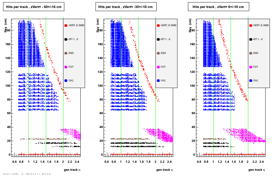
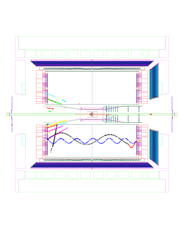
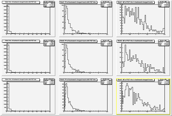
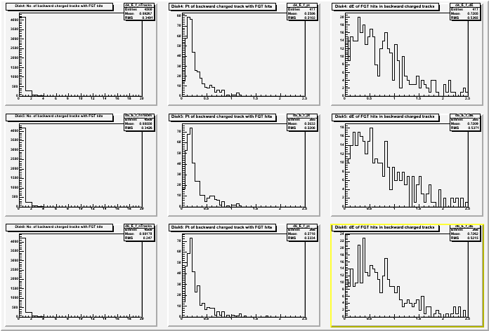
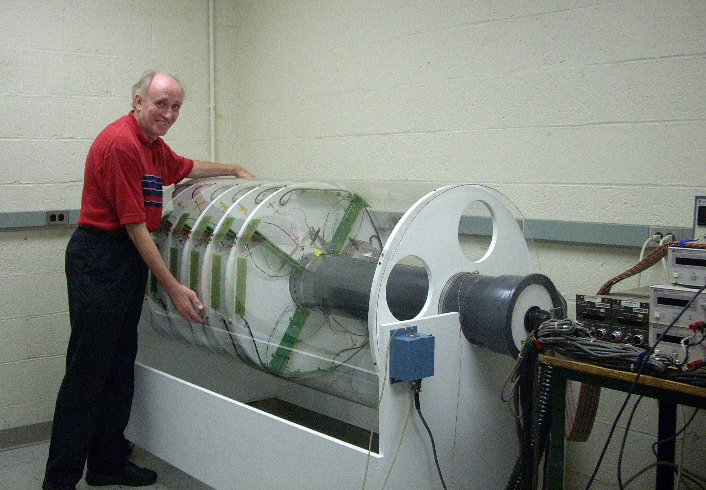
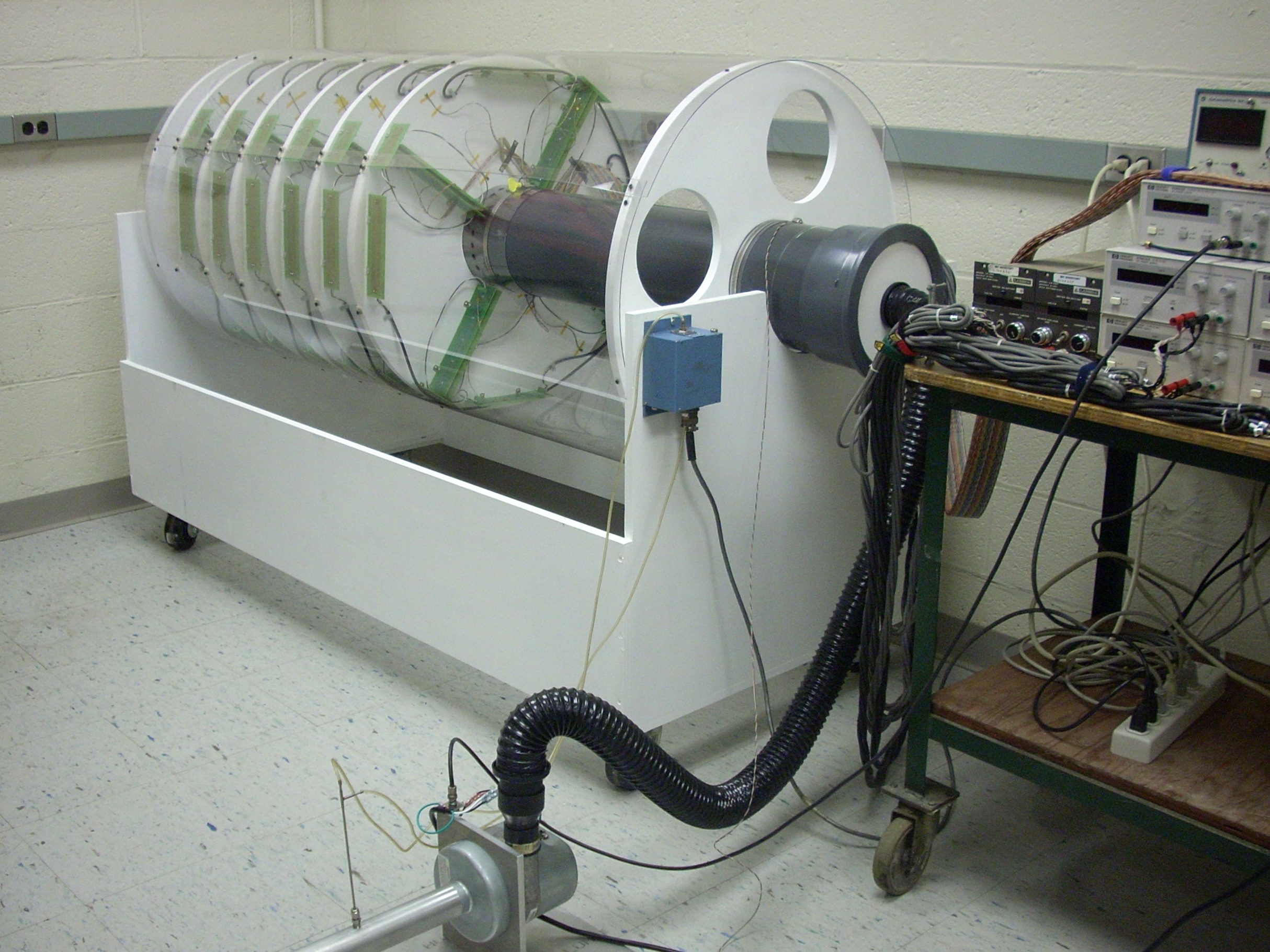
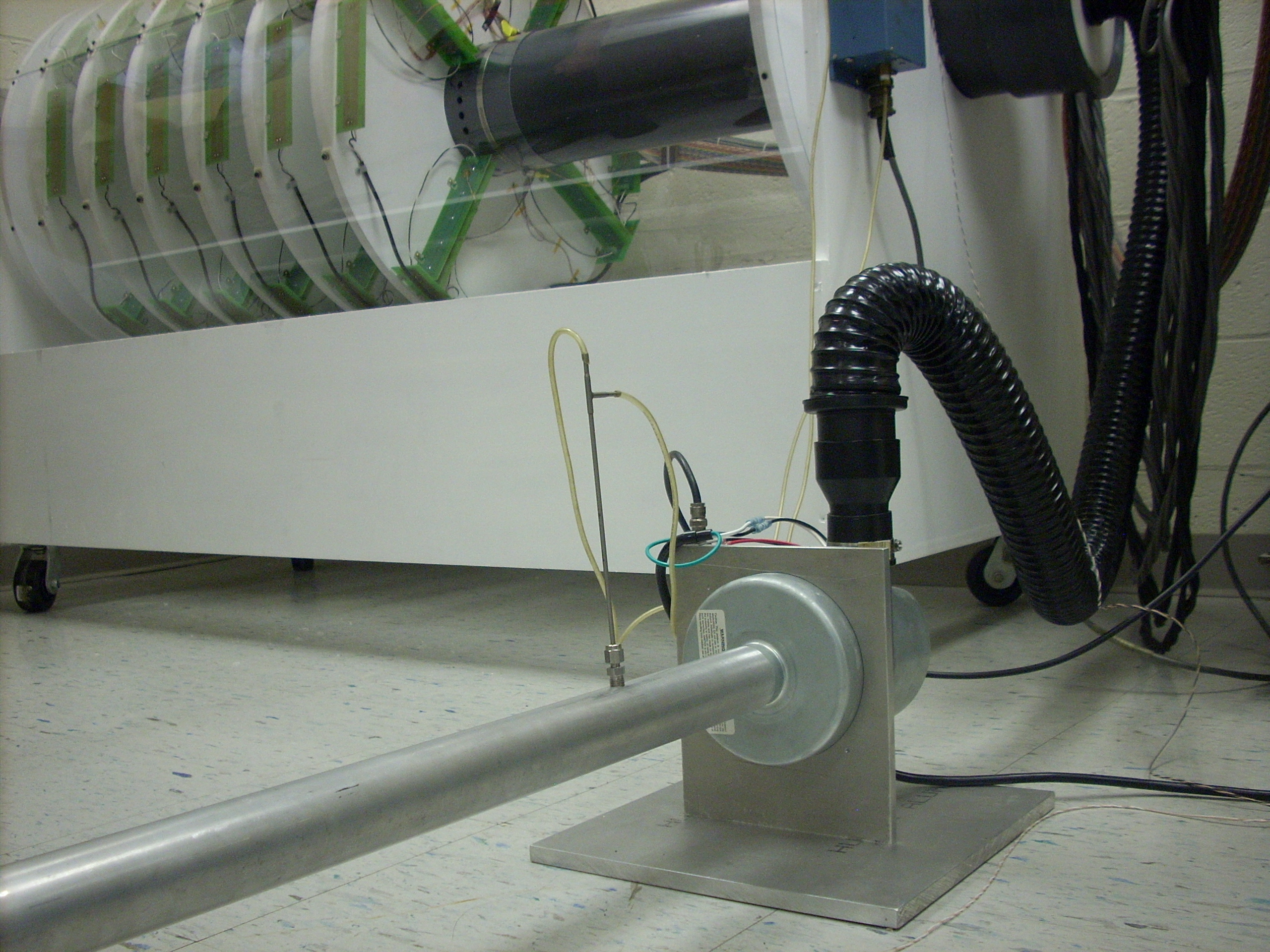
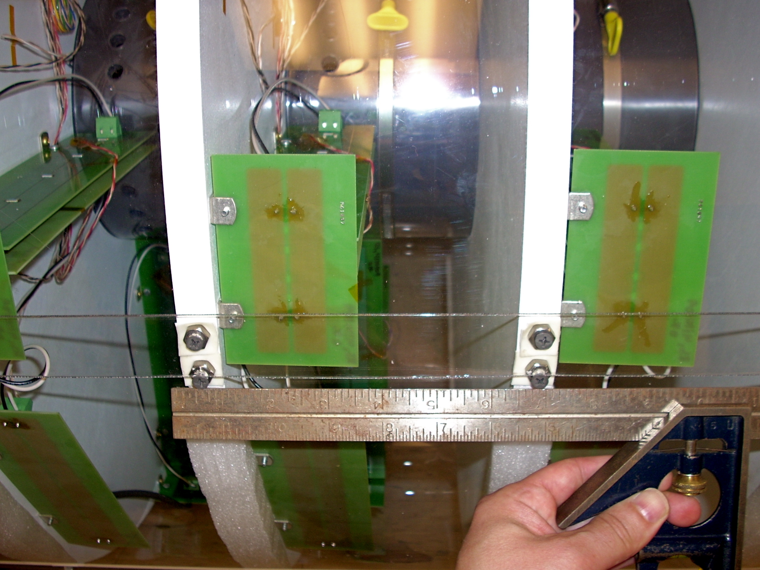
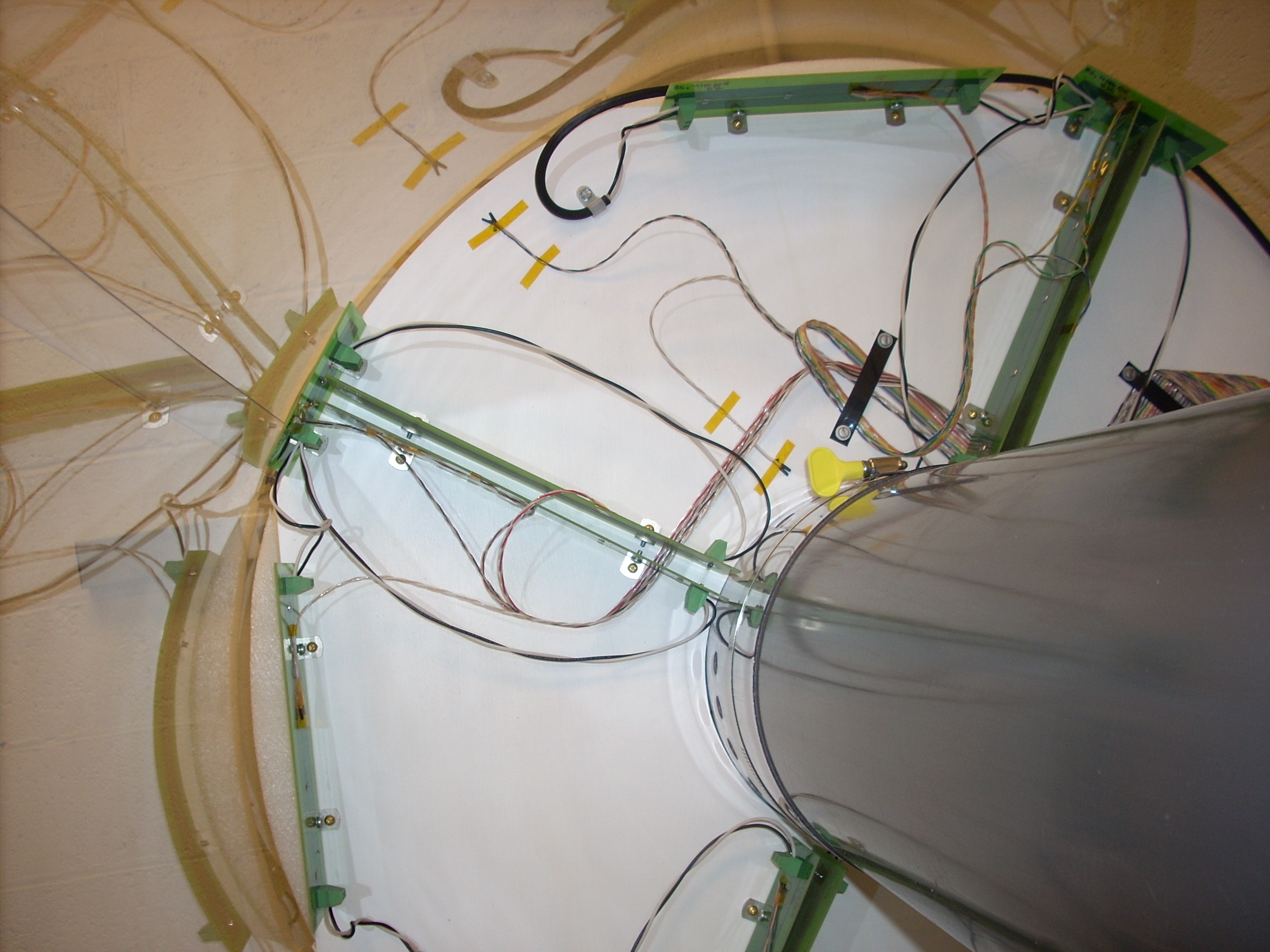
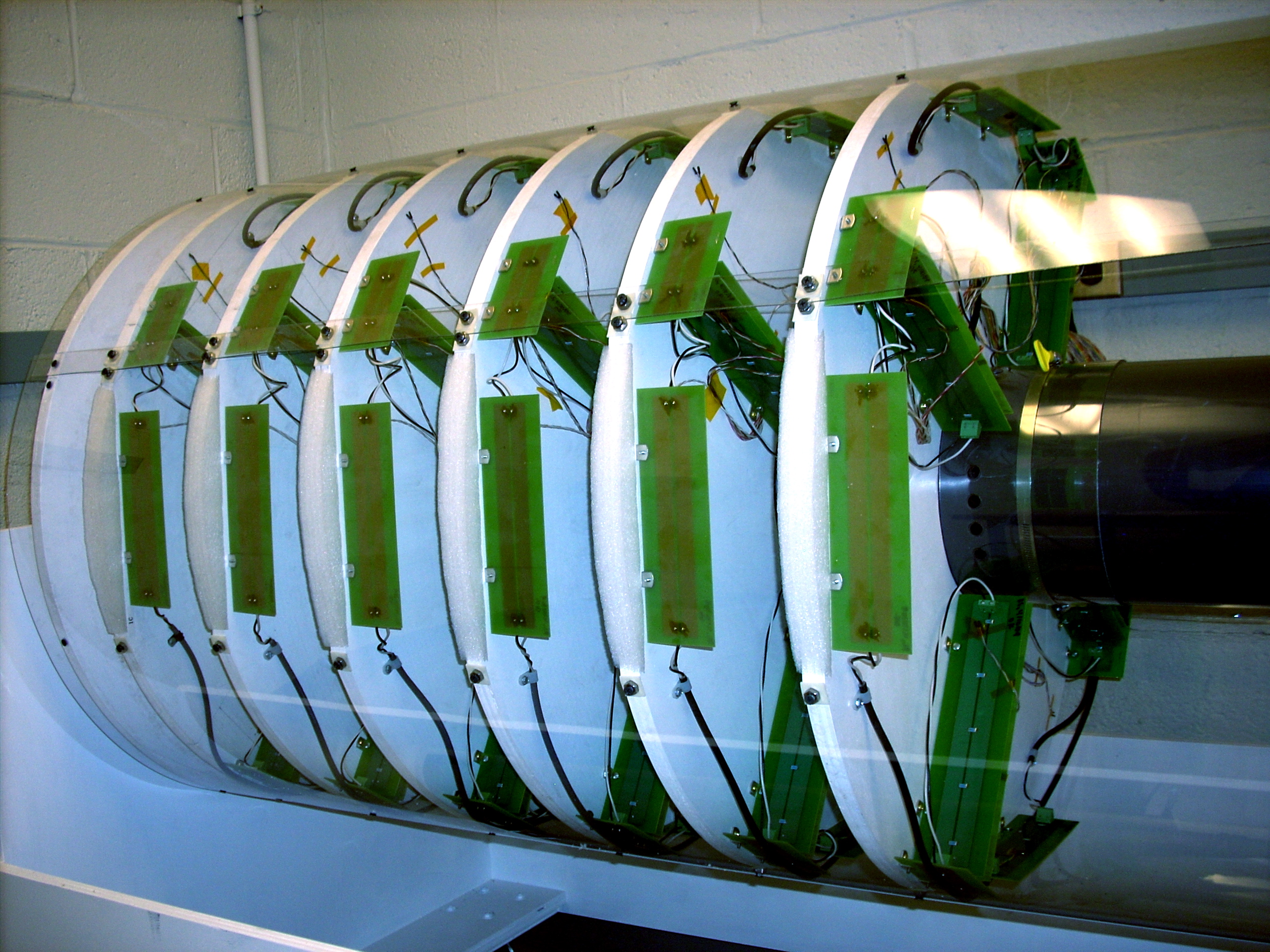
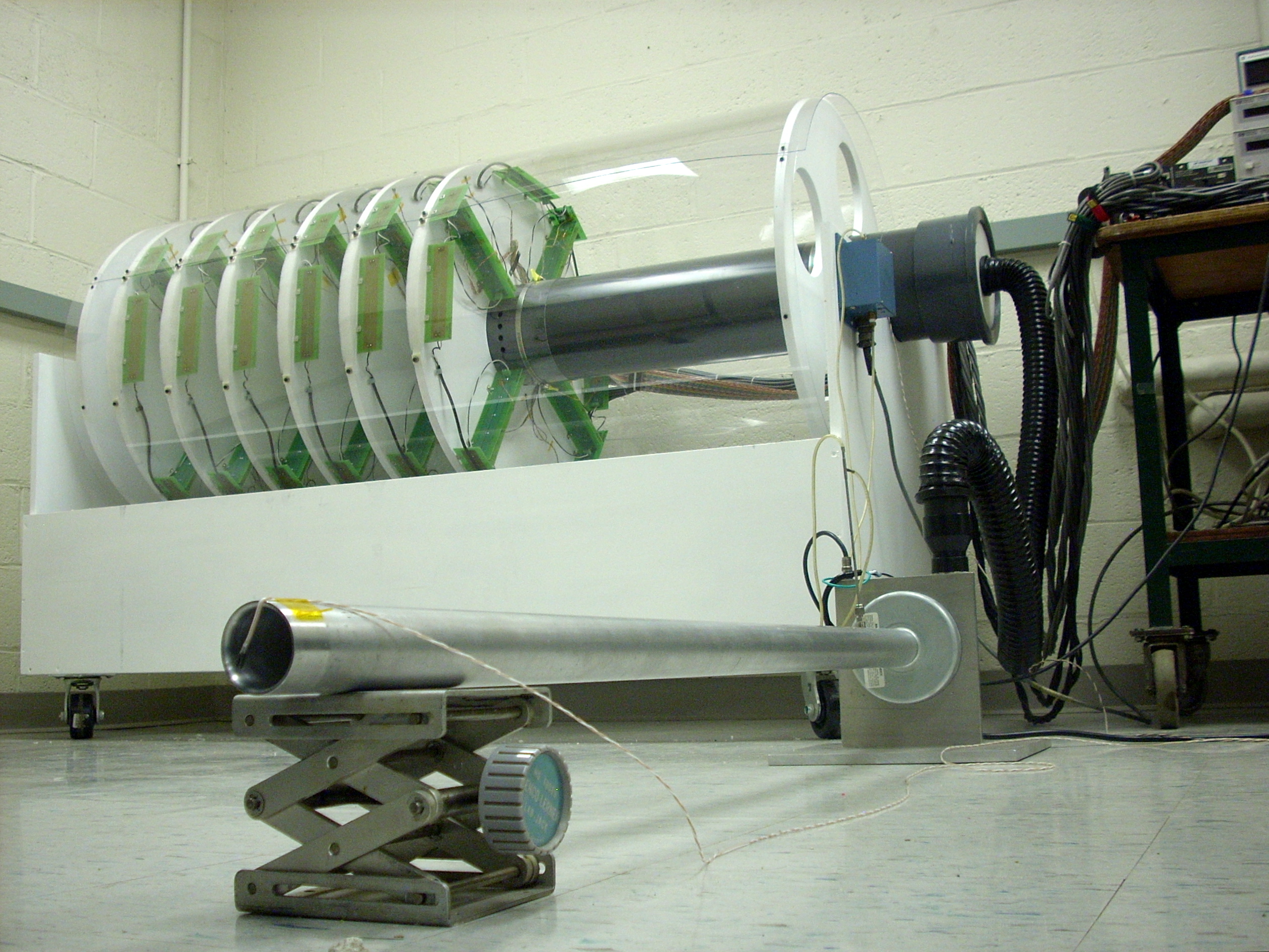
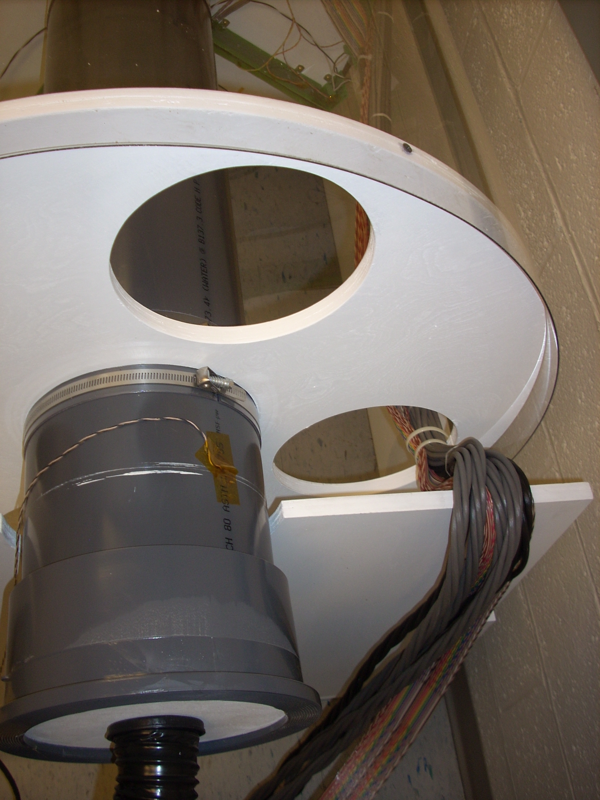
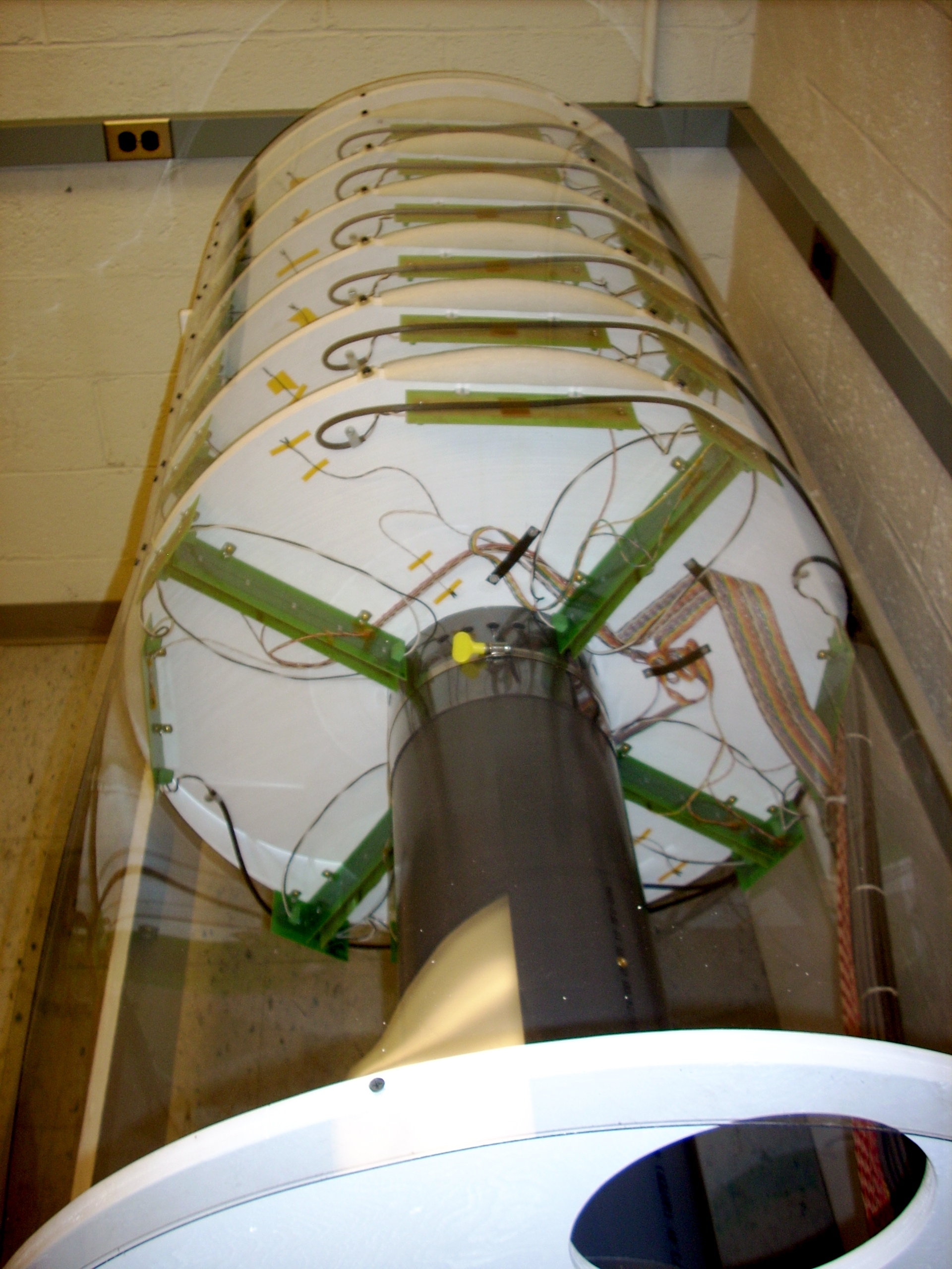
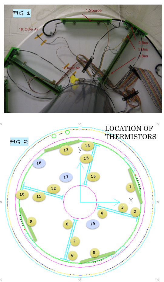
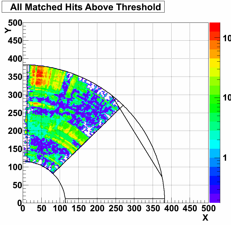
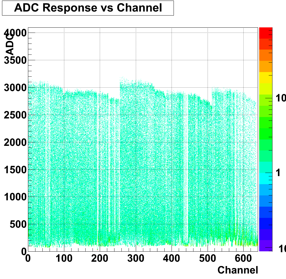
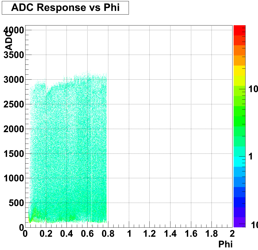
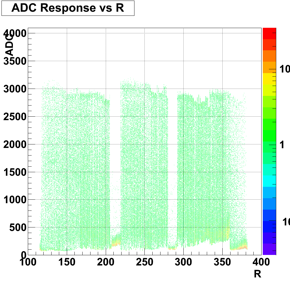
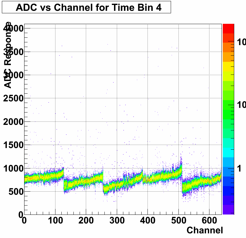
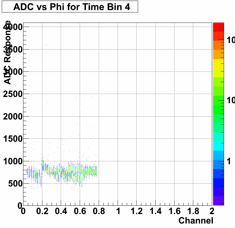
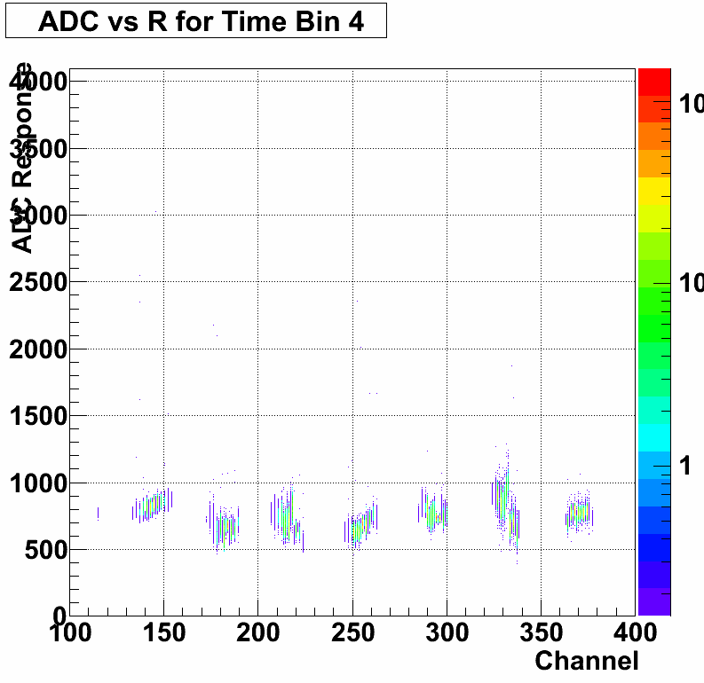
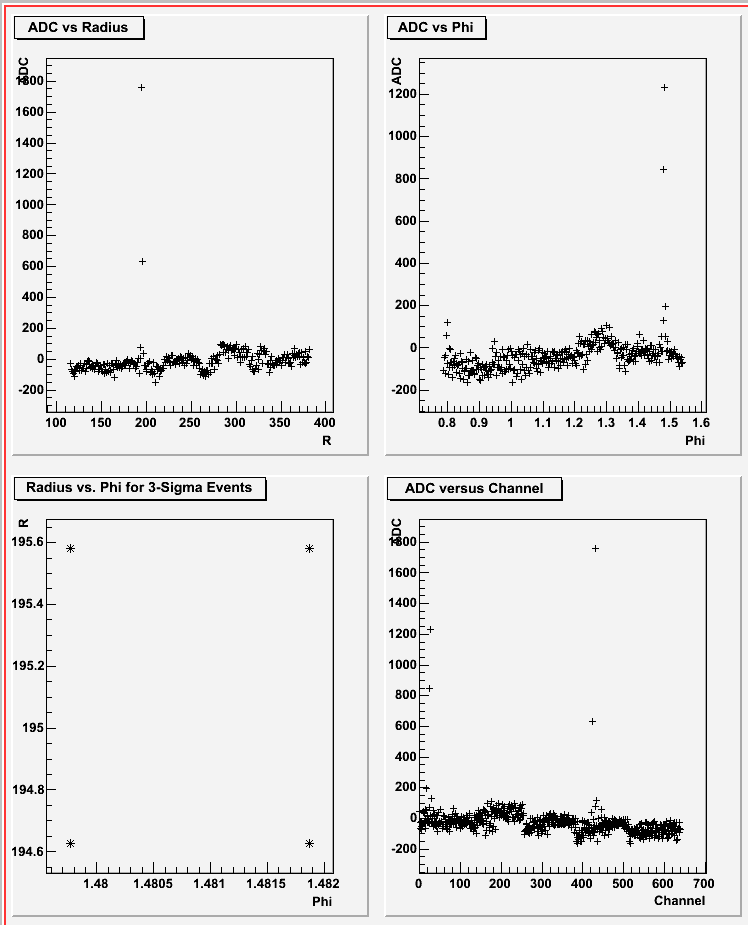
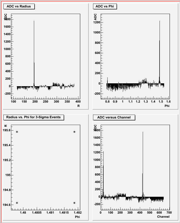
Planned Measurements

Planned Measurements

For each of these measurements we should have a plan/protocoll what we want to do (conditions, time, software...)

• Normal
  0

  false
  false
  false

  EN-US
  X-NONE
  X-NONE

  /* Style Definitions */
  table.MsoNormalTable
  {mso-style-name:"Table Normal";
  mso-tstyle-rowband-size:0;
  mso-tstyle-colband-size:0;
  mso-style-noshow:yes;
  mso-style-priority:99;
  mso-style-parent:"";
  mso-padding-alt:0in 5.4pt 0in 5.4pt;
  mso-para-margin:0in;
  mso-para-margin-bottom:.0001pt;
  mso-pagination:widow-orphan;
  font-size:11.0pt;
  font-family:"Calibri","sans-serif";
  mso-ascii-font-family:Calibri;
  mso-ascii-theme-font:minor-latin;
  mso-hansi-font-family:Calibri;
  mso-hansi-theme-font:minor-latin;
  mso-bidi-font-family:"Times New Roman";
  mso-bidi-theme-font:minor-bidi;}

  Reproduction of test beam results at FNAL:  drupal.star.bnl.gov/STAR/blog/surrow/2011/feb/02/fgt-testbeam-fnal-prototype-triple-gem-detectors

• Cluster reconstruction, Cluster size,
• R-Phi Correlations
• Efficiency
• Cluster amplitude
• HV scans
• Residuals
• Dependence on

  Normal
  0

  false
  false
  false

  EN-US
  X-NONE
  X-NONE

  /* Style Definitions */
  table.MsoNormalTable
  {mso-style-name:"Table Normal";
  mso-tstyle-rowband-size:0;
  mso-tstyle-colband-size:0;
  mso-style-noshow:yes;
  mso-style-priority:99;
  mso-style-parent:"";
  mso-padding-alt:0in 5.4pt 0in 5.4pt;
  mso-para-margin:0in;
  mso-para-margin-bottom:.0001pt;
  mso-pagination:widow-orphan;
  font-size:11.0pt;
  font-family:"Calibri","sans-serif";
  mso-ascii-font-family:Calibri;
  mso-ascii-theme-font:minor-latin;
  mso-hansi-font-family:Calibri;
  mso-hansi-theme-font:minor-latin;
  mso-bidi-font-family:"Times New Roman";
  mso-bidi-theme-font:minor-bidi;}

  on inclination angle for P/Phi reconstruction

• Noise (i.e. electronics noise of the readout). RMS of pedestals calibrated to MIP. Optimum parameters for APV in FGT. (Parameters will affect gain as well as noise, of course.) Necessity (or hopefully not) of tracking pedestals by capid.
•  Number of timebins to use in readout, and algorithm to get pulse amplitude/time from the timebin data. Uniformity of signal shape over the detector.

• Crosstalk

• Normal
  0

  false
  false
  false

  EN-US
  X-NONE
  X-NONE

  /* Style Definitions */
  table.MsoNormalTable
  {mso-style-name:"Table Normal";
  mso-tstyle-rowband-size:0;
  mso-tstyle-colband-size:0;
  mso-style-noshow:yes;
  mso-style-priority:99;
  mso-style-parent:"";
  mso-padding-alt:0in 5.4pt 0in 5.4pt;
  mso-para-margin:0in;
  mso-para-margin-bottom:.0001pt;
  mso-pagination:widow-orphan;
  font-size:11.0pt;
  font-family:"Calibri","sans-serif";
  mso-ascii-font-family:Calibri;
  mso-ascii-theme-font:minor-latin;
  mso-hansi-font-family:Calibri;
  mso-hansi-theme-font:minor-latin;
  mso-bidi-font-family:"Times New Roman";
  mso-bidi-theme-font:minor-bidi;}

  Rate dependence (trigger rate and signal rate).

• Normal
  0

  false
  false
  false

  EN-US
  X-NONE
  X-NONE

  /* Style Definitions */
  table.MsoNormalTable
  {mso-style-name:"Table Normal";
  mso-tstyle-rowband-size:0;
  mso-tstyle-colband-size:0;
  mso-style-noshow:yes;
  mso-style-priority:99;
  mso-style-parent:"";
  mso-padding-alt:0in 5.4pt 0in 5.4pt;
  mso-para-margin:0in;
  mso-para-margin-bottom:.0001pt;
  mso-pagination:widow-orphan;
  font-size:11.0pt;
  font-family:"Calibri","sans-serif";
  mso-ascii-font-family:Calibri;
  mso-ascii-theme-font:minor-latin;
  mso-hansi-font-family:Calibri;
  mso-hansi-theme-font:minor-latin;
  mso-bidi-font-family:"Times New Roman";
  mso-bidi-theme-font:minor-bidi;}

  .Radiation effects on the frontend electronics

• Normal
  0

  false
  false
  false

  EN-US
  X-NONE
  X-NONE

  /* Style Definitions */
  table.MsoNormalTable
  {mso-style-name:"Table Normal";
  mso-tstyle-rowband-size:0;
  mso-tstyle-colband-size:0;
  mso-style-noshow:yes;
  mso-style-priority:99;
  mso-style-parent:"";
  mso-padding-alt:0in 5.4pt 0in 5.4pt;
  mso-para-margin:0in;
  mso-para-margin-bottom:.0001pt;
  mso-pagination:widow-orphan;
  font-size:11.0pt;
  font-family:"Calibri","sans-serif";
  mso-ascii-font-family:Calibri;
  mso-ascii-theme-font:minor-latin;
  mso-hansi-font-family:Calibri;
  mso-hansi-theme-font:minor-latin;
  mso-bidi-font-family:"Times New Roman";
  mso-bidi-theme-font:minor-bidi;}

   EMI issues. (For the most part if there are any, have to be

   addressed first and independently of the rest of the testing, test

  beam or otherwise.)

• Normal
  0

  false
  false
  false

  EN-US
  X-NONE
  X-NONE

  /* Style Definitions */
  table.MsoNormalTable
  {mso-style-name:"Table Normal";
  mso-tstyle-rowband-size:0;
  mso-tstyle-colband-size:0;
  mso-style-noshow:yes;
  mso-style-priority:99;
  mso-style-parent:"";
  mso-padding-alt:0in 5.4pt 0in 5.4pt;
  mso-para-margin:0in;
  mso-para-margin-bottom:.0001pt;
  mso-pagination:widow-orphan;
  font-size:11.0pt;
  font-family:"Calibri","sans-serif";
  mso-ascii-font-family:Calibri;
  mso-ascii-theme-font:minor-latin;
  mso-hansi-font-family:Calibri;
  mso-hansi-theme-font:minor-latin;
  mso-bidi-font-family:"Times New Roman";
  mso-bidi-theme-font:minor-bidi;}

  Optimum gain setting for the FGT in consideration of the limited dynamic range of APV. What tail of large events can we afford to cut off and still make the position resolution? Conversely how much noise is affordable and still make the position resolution. Presumably get to a plot of resolution as a function of HV setting.

• Normal
  0

  false
  false
  false

  EN-US
  X-NONE
  X-NONE

  /* Style Definitions */
  table.MsoNormalTable
  {mso-style-name:"Table Normal";
  mso-tstyle-rowband-size:0;
  mso-tstyle-colband-size:0;
  mso-style-noshow:yes;
  mso-style-priority:99;
  mso-style-parent:"";
  mso-padding-alt:0in 5.4pt 0in 5.4pt;
  mso-para-margin:0in;
  mso-para-margin-bottom:.0001pt;
  mso-pagination:widow-orphan;
  font-size:11.0pt;
  font-family:"Calibri","sans-serif";
  mso-ascii-font-family:Calibri;
  mso-ascii-theme-font:minor-latin;
  mso-hansi-font-family:Calibri;
  mso-hansi-theme-font:minor-latin;
  mso-bidi-font-family:"Times New Roman";
  mso-bidi-theme-font:minor-bidi;}

  Survival of FEE to breakdown/discharges in detector

Test Stand

Deleted Documents

Deleted documents.