- General information
- Data readiness
- Calibration
- BeamLine Constraint
- Calibration Run preparation
- Calibration Schedules
- Calibration topics by dataset
- Docs
- STAR Automated Calibration Project
- SVT Calibrations
- TPC Calibrations
- Drift velocity
- Enter TPC gains into database
- Field Cage Shorts
- Miscellaneous TPC calibration notes
- Padrow 13 and Padrow 40 static distortions
- RunXI dE/dx calibration recipe
- SpaceCharge and GridLeak
- SpaceCharge and GridLeak Calibration How-To Guide
- Effect of SVT and SSD on SpaceCharge Calibration
- SpaceCharge azimuthal anisotropy
- AuAu15 (2014)
- AuAu19 (2011)
- AuAu200 (2004)
- AuAu200 (2007)
- AuAu200 (2011)
- AuAu200 (2014)
- AuAu200 (2016)
- AuAu27 (2011)
- CuAu200 (2012)
- CuCu200 (2005)
- CuCu22 (2005)
- GridLeak R&D
- UU193 (2012)
- dAu20 (2016)
- dAu200 (2008)
- dAu200 (2016)
- dAu39 (2016)
- dAu62 (2016)
- pAl200 (2015)
- pAu200 (2015)
- pp200 (2006)
- pp200 (2009)
- pp200 (2015)
- pp400 (2005)
- pp500 (2011)
- pp510 (2012)
- pp510 (2013)
- pp62 (2006)
- TPC Hit Errors
- TPC OmegaTau
- TPC Sector Alignment
- TPC Slewing
- TPC T0s
- TPC de/dx
- TPC survey instructions
- Twist (ExB) Distortion
- Databases
- Quality Assurance
- Calibration
- Grid and Cloud
- Infrastructure
- Machine Learning
- Offline Software
- Production
- S&C internal group meetings
- Test tree
SpaceCharge and GridLeak Calibration How-To Guide
Updated on Wed, 2012-12-19 14:58. Originally created by genevb on 2006-01-06 15:30.
Under:
The following steps explain how to perform the calibrations of the SpaceCharge and GridLeak database entries. There are many steps, but they should be straightforward and not quite as difficult as the length of this document might imply. For further information, please contact Gene Van Buren.
- SETUP
- Make sure sufficient DAQ files for this dataset are available.
Somewhere around 30 to 50 DAQ files will probably do fine, with collisions producing small multiplicities needing the most DAQ files (e.g. pp collisions will need about 50 DAQ files). These DAQ files should represent a large spread in the collider luminosity. Randomly picking files scattered throughout the dataset run period will probably suffice, but this should be checked by looking at the range that the scalers cover during the first pass (see below).
- Determine the timestamp and magnetic field that will be used for this data.
You can use the RunLog Browser to determine the date and time of the first acquired data, as well as the magnetic field setting (reversed, half, etc.).
- Choose a working directory.
You will need plenty of disk space for histograms (perhaps 1 GB).
- Create local database values for SpaceCharge and GridLeak.
When the chain runs, it will first look for local versions (in a directory call StarDb) of the tables it wants from the database. We will need several versions of this directory, so it is wise to choose meaningful names. I like to make directories named StarDbX_Y, where X and Y are the SpaceCharge and GridLeak values I use.
Inside this directory, there need to be two files:
* spaceChargeCorR2.20071101.000001.C
* StarDbX_Y/Calibrations/tpc/tpcGridLeak.DDDDDDDD.TTTTTT.C
where DDDDDDDD.TTTTTT is the appropriate timestamp for this data. Example versions of those files are available by clicking on the each of the above filenames. - Create directories for histograms.
Again, we will need several directories, so naming wisely helps. I like to use the names histsX_Y, with X and Y as with StarDb.
- Decide on the chain to use.
This should be the analysis chain, with a few modifcations:
- SCScalerCal, OSpaceZ2, and OGridLeak3D options should be turned on.
- Use of any inner-tracking detectors should be switched off. I've found that the following options turn off the SVT: "-svtD -svtdEdx -SvtIT".
- Create a script to use with the scheduler.
This script will need to provide the jobs with the appropriate StarDb data, and the appropriate place to put the histograms. I have been doing this with soft links, as can be seen in my current example script(this is the runCalib.xml script attached to this page: your browser may not show it well, so download it or view source), but this should be updated with use of the sandbox and output elements at some point.
- Make sure sufficient DAQ files for this dataset are available.
- FIRST PASS
In this pass, we will use zero space charge to analyze the data, and see what the calibration code recommends we should use for the space charge. These are the steps to proceed:
VERY IMPORTANT NOTE: This is unlikely to work as desired any more! When luminosities are so high that data uncorrected for SpaceCharge and GridLeak causes significant track splitting at the inner/outer TPC sector boundaries, such data is not useful for calibration. In such cases (perhaps all cases, now that luminosities are higher), the first pass should be made with a reasonable guess for the value of SpaceCharge based on historical values. It is still value to read these instructions and understand the concept of producing data, obtaining results, and getting improved guesses from there.
- Create three StarDb directories for zero SpaceCharge.
Set up three StarDb directories as described earlier with GridLeak values of 9.0, 12.0, and 15.0. I would label these directories StarDb0_9.0, StarDb0_12.0, and StarDb_15.0. Edit the SpaceCharge files so that the appropriate line has the value 0 (e.g. row.fullFieldB = 0 for Reversed Full Field data). The other values don't matter just yet. The GridLeak files should also have a single line edited (e.g. row.MiddlGLStrength = 9.0, etc.).
- Create three histogram directories.
For these three sets, I use hists0_9.0, hists0_12.0, hists0_15.0.
- Edit the scheduler script to use the correct StarDb and hists directories and run the script.
I just edit the script for one set of values, run it, and then edit, run, edit, run.
- Check that the histograms are getting created.
When the jobs are finished running, the hists directories should have a histogram file for each of the jobs run. Don't worry if a few don't turn up or finish. These histogram files contain a variety of histograms and a TTree called SC.
- Look at the range covered by the scalers to make sure this is a sufficient spread in luminosity.
You will need to decide for yourself if this is true by looking, for example, at the histogram produced by the following:
If this plot looks more like a blob than a somewhat linear distribution, it is unlikely that there is enough spread in luminosity. You should specifically try to include more DAQ files at different luminosities. You will then need to run the first pass on those new files, and they will simply add more histograms in your hists directories.root -l
[0] TChain SC("SC")
[1] SC.Add("hists0_12.0/*")
[2] SC.Draw("sc:zdcx")This is also a good time to see if there are some obvious outliers in the data which should not be used in the calibration proceedure. The variable "run" is available from the TTree/TChain, so you might find, for example that all the data from run 1366001 is looks weird and you can cut on these later.
- Create an input file for the Calib_SC_GL.C macro.
Instructions for the input file are found in the header of the macro (documentation), but for this first pass, it will look something like this:
hists0_9.0/*  0 0 9.0
hists0_12.0/* 0 0 12.0
hists0_15.0/* 0 0 15.0 - Run the macro on the input file.
If the file is named input.dat, then execute:
If there was a run you wanted to exclude, you might execute:root -l 'Calib_SC_GL.C("input.dat")'root -l 'Calib_SC_GL.C("input.dat","run!=1366001")' - The macro will output suggestions for further passes.
The output might look like this:
The first important line is that the calibration code determined the scaler which shows the tightest correlation with SpaceCharge. This is the scaler which should be used from here on as the scaler to which we will calibrate, and the ID is the number you will need to enter for row.detector in the local SpaceCharge database file.Found 3 dataset specifications.
*** Best scaler = bbce+bbcw [ID = 4]
*** Try the following calibration values: ***
SC = 1.39e-08 * ((bbce+bbcw) - (2.39e+04)) with GL = 9.0
SC = 1.32e-08 * ((bbce+bbcw) - (2.08e+04)) with GL = 12.0
SC = 1.18e-08 * ((bbce+bbcw) - (2.23e+04)) with GL = 15.0The next lines suggest values to use in the next pass of calibration. (and the histograms just display these values). The multiplicative factor goes into the local SpaceCharge database file where you put 0 before, and the subtracted offset goes in the row.offset value.
- Create three StarDb directories for zero SpaceCharge.
- ITERATIVE PASSES
- Create local StarDb and GridLeak files for the new values.
The first pass will output suggestions for these values, and you can simply use these. Other passes will only output one suggestion, but you'll get good results if you use at least 3 possibilities. So I recommend using the suggested SpaceCharge values, and then three different GridLeak values: the suggested one, and perhaps plus and minus 1.0 from that value. It is not important to get these values exactly correct to some particular number, but it is good to get them close to the final calibration so that they provide better constraint in the fitting routines.
- Edit and run the scheduler script as before.
- Edit the input file (or create a new one) for the macro.
You can keep the previous pass histogram datasets in the input file, and simply add more lines for each of the new datasets. More data means a more accurate fit.
- Run the macro on the input file as before, with any cuts as before.
Because you have already decided upon a scaler to use, you can make the macro run faster by limiting it to only look at that specific scaler. The third argument of the macro does this. So for bbce+bbcw, you might execute something like:
root -l 'Calib_SC_GL.C("input2.dat","run!=1366001&&run!=1987654",4)' - The macro will output a suggested calibration value.
The output of the macro in any of these subsequent passes will look something like this:
The first few lines are simply outputs from the fitting procedures, which correspond to the information shown in the plots. After a couple iterations, these plots should look something like this:Found 9 dataset specifications.
* Constraint on SC x GL = 1.17e-07
* Guesses on SC = 1.39e-08 , 6.45e-09 , 1.4e-08 , 6.45e-09
* Guesses on SO = 2.4e+04 , 2.35e+04
*** FINAL CALIBRATION VALUES: ***
SC = 1.4e-08 * ((bbce+bbcw) - (2.37e+04)) with GL = 8.3
For the most part, the plots should not be too much of a concern unless some of the datapoints seem to fall very far from the fit curves (a few sigma away, perhaps), in which case there may be some data causing the fits to act weirdly and you should again look for obvious outliers which might be doing this.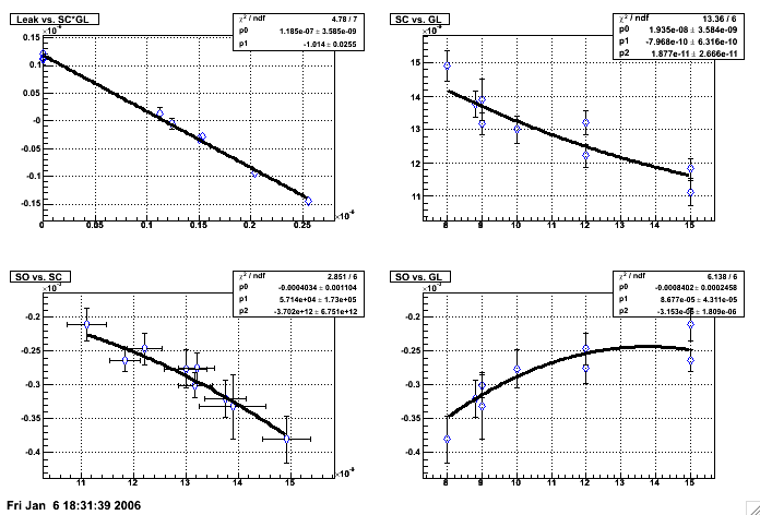
The last line shows the suggested final calibration value.
- Decide whether to iterate on another pass.
After a few iterations, the final calibration values should be stable. This is a sign that you can stop the procedure and use those values. If this is not stabilizing within a few passes, you will need to figure out why.
- Create local StarDb and GridLeak files for the new values.
- FINISH
- You may want to take a look at more detailed GridLeak plots using the final calibration values, but this is another topic.
- If you're happy, submit the final calibration values to the database.
- Archive and document your work!
- Relax - you're done.
»
- Printer-friendly version
- Login or register to post comments