Cut optimization with Fisher's LDA and MLP (neural network) classifiers

ROOT implementation for LDA and MLP:

• Fisher's Linear Discriminant Analysis (LDA)
• Multi-Layer Perceptron (MLP) [feed-forward neural network]

Application for cuts optimization in the gamma-jet analysis

LDA configuration: default

MLP configuration:

• 2 hidden layers [N+1:N neural network configuration, N is number of input parameters]
• Learning method: stochastic minimization (1000 learning cycles)

Input parameters (same for both LDA and MLP):

1. Energy fraction in 3x3 cluster within a r=0.7 radius: r3x3
2. Photon-jet pt balance: [pt_gamma-pt_jet]/pt_gamma
3. Number of charge tracks within r=0.7 around gamma candidate
4. Number of Endcap towers fired within r=0.7 around gamma candidate
5. Number of Barrel towers fired within r=0.7 around gamma candidate

Figure 1: Signal efficiency and purity, background rejection (left),
and significance: Sig/sqrt[Sig+Bg] (right) vs. LDA (upper plots) and MLP (lower plots) classifier discriminants

Figure 2:

1. Upper left: Rejection vs. efficiency
2. Upper right: Purity vs. efficiency
3. Lower left: Purity vs. Rejection
4. Lower right: Significance vs. efficiency

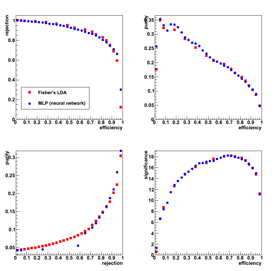
Figure 3: Data to Monte-Carlo comparison for LDA (upper plots) and MLP (lower plots)
Good (within ~ 10%) match between data nad Monte-Carlo
a) up to 0.8 for LDA discriminant, and b) up to -0.7 for MLP.

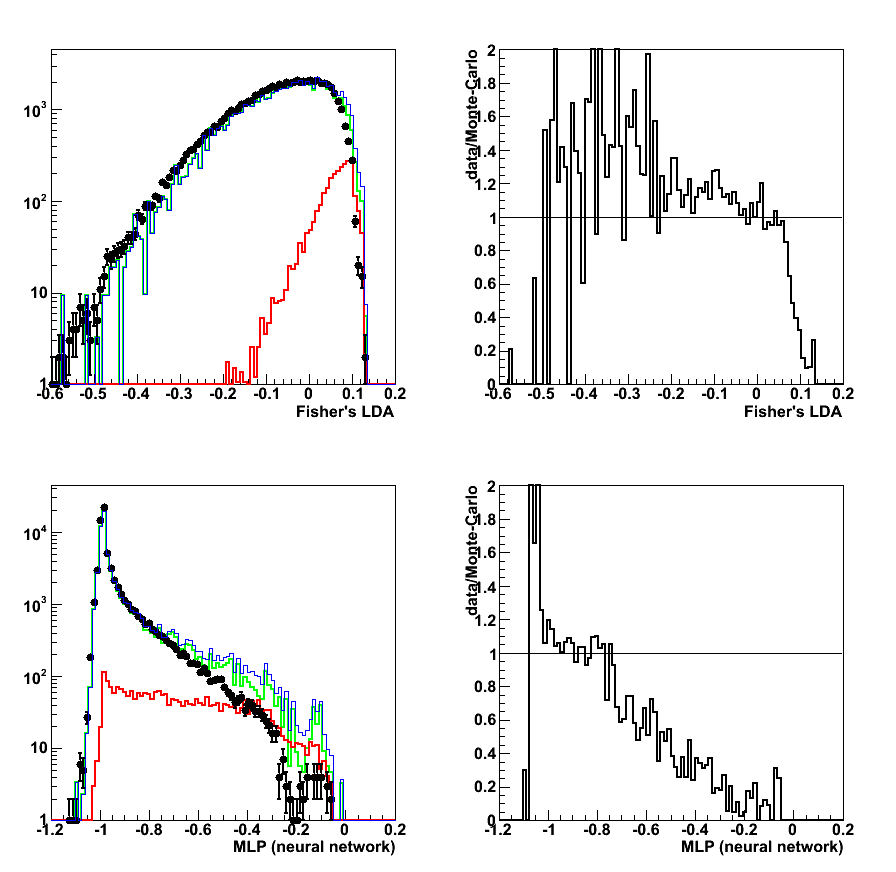
Figure 4: Data to Monte-Carlo comparison for input parameters
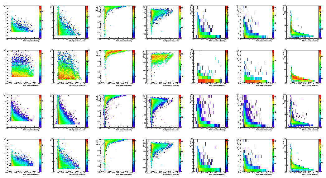
from left to right
1) pt_gamma 2) pt_jet 3) r3x3 4) gamma-jet pt balance 5) N_ch[gamma] 6) N_eTow[gamma] 7) N_bTow[gamma]
Colour coding: black pp2006 data, red gamma-jet MC, green QCD MC, blue gamma-jet+QCD

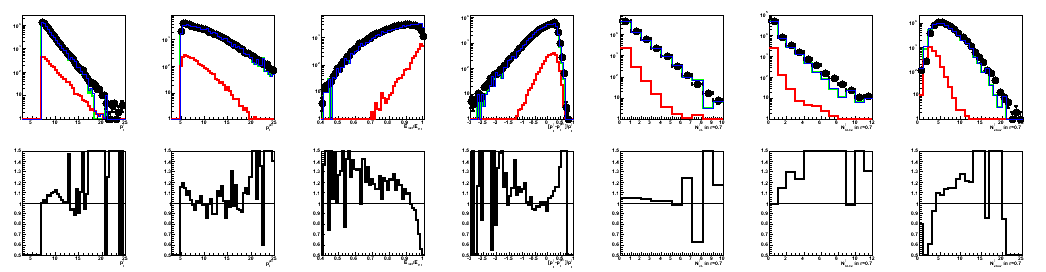
Figure 5: Data to Monte-Carlo comparison:
correlations between input variables (in the same order as in Fig. 4)
and LDA classifier discriminant (horizontal axis).
1st raw: QCD MC; 2nd: gamma-jet MC; 3rd: pp2006 data; 4th: QCD+gamma-jet MC

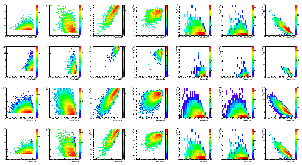
Figure 6: Same as Fig. 6 for MLP discriminant