2008.09.30 Sided residual: purity, efficiency, and background rejection
Ilya Selyuzhenkov September 30, 2008
Data sets:
- pp2006 - STAR 2006 pp longitudinal data (~ 3.164 pb^1)
after applying gamma-jet isolation cuts (note: R_cluster > 0.9 is used below). - gamma-jet - data-driven Pythia gamma-jet sample (~170K events). Partonic pt range 5-35 GeV.
- QCD jets - data-driven Pythia QCD jets sample (~4M events). Partonic pt range 3-65 GeV.
Notations used in the plots:
- Fit peak energy:
F_peak - integral within +-2 strips from maximum strip
Maximum strip determined by fitting procedure.
Float value converted ("cutted") to integer value. - Data peak energy:
D_peak - energy sum within +-2 strips from maximum strip (the same strip Id as for F_peak). - Data tails:
D_tail^left and D_tail^right.
Energy sum from 3rd strip up to 30 strips on the
left and right sides from maximum strip (excludes strips which contributes to D_peak) - Fit tails:
F_tail^left and F_tail^right.
Same definition as for D_tail, but integrals are calculated from a fit function. - Maximum sided residual:
max(D_tail-F_tail)
Maximum of the data minus fit energy on the left and right sides from the peak.
Determining cut line based on sided residual plot
Figure 1: Sided residual plot: D_peak vs. max(D_tail-F_tail)
Red lines show 4th order polynomial functions, a*x^4,
which have 80% of MC gamma-jet counts on the left side.
These lines are obtained independently for each of pre-shower condition
based on fit procedure shown in Fig. 3 below.
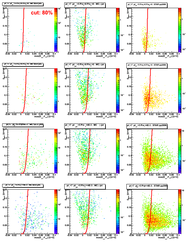
Figure 2: max(D_tail-F_tail) distribution
(projection on horizontal axis from sided residual plot, see Fig. 1 above)
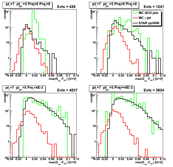
Figure 3: max(D_tail-F_tail) [at 80%] vs. D_peak.
For each slice (bin) in D_peak variable, the max(D_tail-F_tail) value
which has 80% of gamma-jet candidates on the left side are plotted.
Lines represent fits to MC gamma-jet points (shown in red) using different fit functions
(linear, 2nd, 4th order polynomials: see legend for color coding).
Note, that in this plot D_peak values are shown on horizontal axis.
Consequently, to get 2nd order polynomial fit on sided residual plot (Fig. 1),
one needs to use sqrt(D_peak) function.
The same apply to 4th order polynomial function.
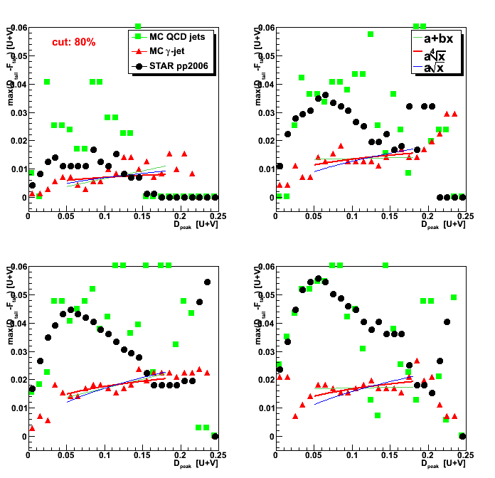
Figure 4: D_peak vs. horisontal distance from 4th order polinomial function to max(D_tail-F_tail) values.
(compare with Fig. 1: Now 80% of MC gamma-jet counts are on the left side from vertical axis)
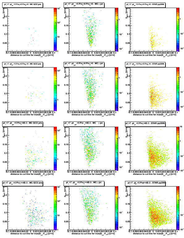
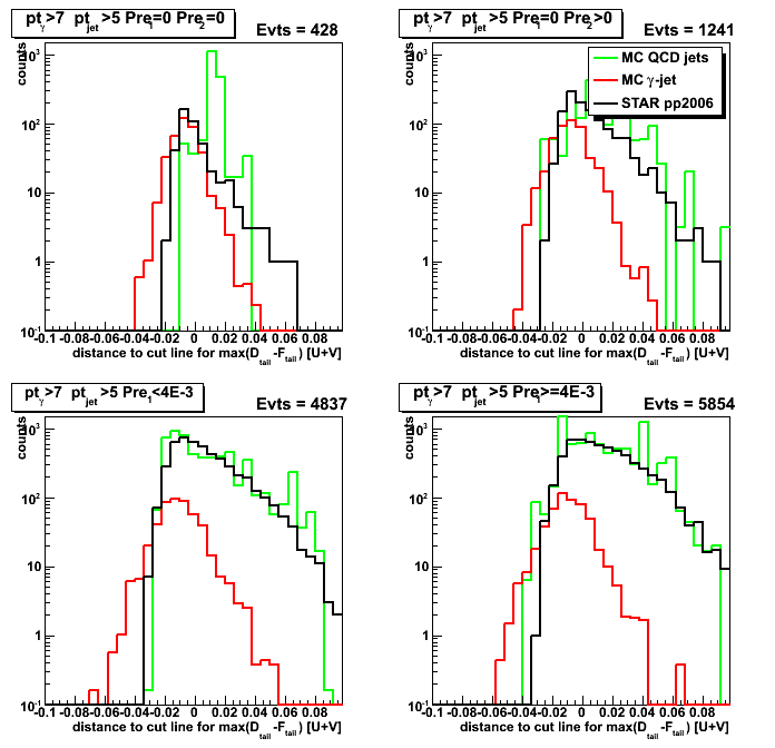
Figure 5: Horizontal distance from 4th order polynomial function to max(D_tail-F_tail)
[Projection on horizontal axis from Fig. 4]
Based on this plot one can obtain purity, efficiency, and rejection plots (see Fig. 6 below)
Gamma-jet purity, efficiency, and QCD background rejection
Horizontal distance plotted in Fig. 5 can be used as a cut
separating gamma-jet signal and QCD-jets background,
and for each value of this distance one can define
gamma-jet purity, efficiency, and QCD-background rejection:
-
gamma-jet purity is defined as the ratio of
the integral on the left for MC gamma-jet data sample, N[g-jet]_left,
to the sum of the integrals on the left for MC gamma-jet and QCD jets, N[QCD]_left, data samples:
Purity[gamma-jet] = N[g-jet]_left/(N[g-jet]_left+N[QCD]_left) -
gamma-jet efficiency is defined as the ratio of
the integral on the left side for MC gamma-jet data sample, N[g-jet]_left,
to the total integral for MC gamma-jet data sample, N[g-jet]:
Efficiency[gamma-jet] = N[g-jet]_left/N[g-jet] -
QCD background rejection is defined as the ratio of
the integral on the right side for MC QCD jets data sample, N[QCD]_right,
to the total integral for MC QCD jets data sample, N[QCD]:
Rejection[QCD] = N[QCD]_right/N[QCD]
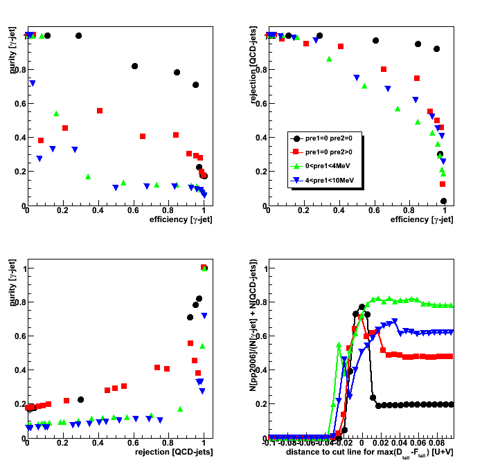
Figure 6: Shows:
purity[g-jet] vs. efficiency[g-jet] (upper left);
rejection[QCD] vs. efficiency[g-jet] (upper right);
purity[g-jet] vs. rejection[QCD] (lower left);
pp2006 to MC ratio, N[pp2006]/(N[g-jet]+N[QCD]), vs. horizontal distance from Fig. 5 (lower right)
- Printer-friendly version
- Login or register to post comments