BEMC
The STAR Barrel Electromagnetic Calorimeter
BEMC Detector Operator Manual
Authored by O. Tsai, 04/13/2006 (updated 02/02/2011)
You will be operating three detectors:
| BTOW | Barrel Electromagnetic Calorimeter |
| BSMD | Barrel Shower Maximum Detector |
| BPSD | Barrel Preshower Detector |
All three detectors are delicate instruments and require careful and precise operation.
It is critical to consult and follow the “STAR DETECTOR STATES FOR RUN 11”
and “Detector Readiness Checklist” for instructions.
Rule 1: If you have a concern of what you are going to do with any of these detectors please don’t hesitate to ask people around you in the control room or call experts to get help or explanations.
This manual will tell you:
- how to turn On/Off low and high voltages for all three detectors.
- how to prepare BTOW for “Physics”.
- how to recover from a PMT HV Trip.
- how to deal with common problems.
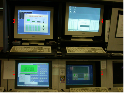
First, familiarize yourself with the environment of the control room. This is a picture of the four terminal windows which you will be using to operate the BEMC systems. For run 11, Terminal 4 is not in use. Terminal 0 (not shown) is on the left side of terminal 1/
(clicking on a link will take you directly to that section in the manual)
0 - (on beatrice.starp.bnl.gov)
1 - (on emc02.starp.bnl.gov)
BEMC PMT Low Voltage Power Supply Slow Control
2 - (on emcsc.starp.bnl.gov)
BTOW HV Control
3 - (on hoosier.starp.bnl.gov)
BSMD HV Control
0 - (on emc01.starp.bnl.gov)
BPSD HV Control
To login on any of these computers use the emc account with password (check the control room copy of the manual).
Terminal 0 “BEMC Main Control Window”
Usually this terminal is logged on to beatrice.starp.bnl.gov
The list of tasks which you will be doing from this terminal is:
- Prepare BEMC detectors for Physics.
- Turning On/Off low voltages on FEEs.
- Turning On/Off BEMC crates.
- Resetting Radstone Boards (HDLC).
- Explain to experts during phone calls what you see on some of the terminals.
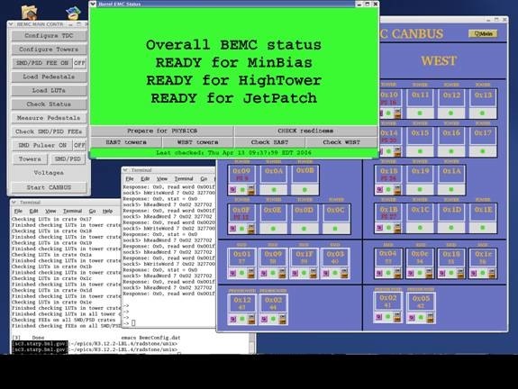
The screenshot above shows how the display on emc02.starp.bnl.gov usually looks during the run. There are five windows open all the time. They are:
- “Barrel EMC Status” - green.
- “BEMC MAIN CONTROL” – gray.
- “BARREL EMC CANBUS” – blue.
- Terminal on sc5.starp.bnl.gov (referred to as the ‘sc5 window’)
- Terminal from telnet scserv 9039 (referred to as ‘HDLC window’)
Prepare BEMC detectors for PHYSICS.
In normal operation this is a one click operation.
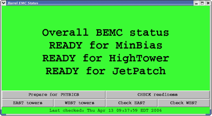
Click “Prepare for PHYSICS” button and in about 10 minutes “Barrel EMC Status” window will turn green and tell you that you are ready to run. This window may look a little bit different from year to year depending trigger requirements for BTOW.
However if this window turns red, then you will be requested to follow the suggested procedures which will popup on this window: simply click on these procedures to perform them.
During “prepare for physics” you can monitor the messages on the sc5 window. This will tell you what the program is actually doing. For example, when you click “Prepare for Physics” you will start a multi-step process which includes:
- Turning OFF FEEs on all SMD/PSD crates
- Programming TDC (Tower Data Collector, Crate 80)
- Reprogramming FPGAs on all BTOW crates
- Configuring all BTOW crates
- Configuring all SMD/PSD FEEs
- Loading pedestals on all BTOW crates
- Loading LUTs on all BTOW crates (only for pp running)
- Checking BTOW crate configuration
- Checking SMD/PSD configuration
- Checking that pedestals were loaded correctly (optional)
- Checking that LUTs were loaded correctly (only for pp running)
Usually, you will not be asked to use any other buttons shown on this window.
BEMC MAIN CONTROL
You can initiate all steps outlined above manually from the BEMC MAIN CONTROL window shown below, and do much more with the BEMC system. However, during normal operation you will not be asked to do that, except in cases when an expert on the phone might ask you to open some additional window from this panel and read back some parameters to diagnose a problem.
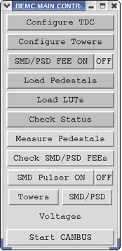
You might be asked to:
- Turn OFF or ON SMD/PSD FEE
- Open SMD/PSD panel and read voltages and currents on different SMD/PSD FEEs
- Open East or West panels to read voltages on some BTOW crates. (Click on Voltages)
That will help experts to diagnose problems you are calling about.
BARREL EMC CANBUS
From this window you can turn Off and On BEMC crates, read parameters of VME crates. This screenshot shows you this window during normal operation with all BEMC crates being ON.
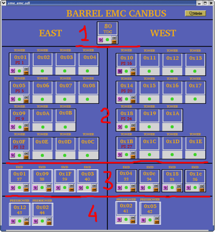
- Crate 80 TDC (Tower Data Collector and “Radstone boards”)
- Thirty crates for BTOW
- Eight crates for BSMD
- Four crates for BPSD
The BTOW crates are powered in groups of three or four from a single power supply (PS) units. The fragment below explains what you see.
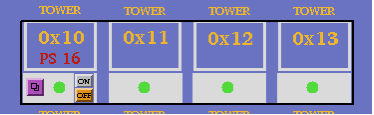
Tower crates 0x10, 0x11, 0x12, 0x13 are all powered from a single power supply: PS 16.
Thus, by clicking the On and Off buttons you will be switching On/Off all four crates and the communication with PMT boxes which are associated with them. (see details in Tower HV Control GUI description).
Sc5 and HDLC windows.
Two other terminal windows on “Terminal 0” are the so-called sc5, and HDLC windows.
These need to be open at all times. To open the sc3 terminal you will need to login as sysuser on sc5.starp.bnl.gov with password (check the control room copy of the manual).
From this sc5 terminal you run two programs. The first program is emc.tcl. If you need for some reason to restart “BEMC MAIN CONTROL” or “Barrel EMC Status” GUI you need to start emc.tcl: the alias for this is emc. To kill this program use alias kill_emc.
To open “Barrel EMC Canbus” GUI use alias emc_canbus_noscale.
If you need to reboot canbus then:
- open sc5 window
- telnet scserv 9040
- press “Ctrl” and “x” keys
- wait while canbus reboots (~5 minutes or so)
- press “Ctrl” and “]” keys
- quit telnet session
- close sc5 window
To open an HDLC window, first you need to open an sc3 window and then telnet scserv 9039.
To close telnet session you need to press “Ctrl” and “]”, and then quit from telnet.
You may be asked by experts on the phone to reset the radstone boards. This is why you need this window open. There are two radstone boards and to reset them type:
radstoneReset 0
and
radstoneReset 1
Terminal 1. “BEMC PMT Low Voltage Power Supply Slow Control”
There is a change in operation procedures for Run7 for PMT HV Low Voltage power supplies.
There are two low voltage power supply PL512 units which powers PMT bases.
PL512 with IP address 130.199.60.79 powers West side and PL512 with IP address 130.199.60.81 powers East side of the detector. A single power supply feeds thirty PMT boxes. The GUI for both PL512 should be open all time on one of the workspace on Terminal1. A screenshot below shows GUI at normal conditions. Both PL512 should be ON all the time, except the case when power cycling of the PMT bases is required.
There are two buttons to turn power On and Off, as usual, wait 30 sec. after turning power supply Off before you will turn it On again. To start GUI use aliases bemc_west and bemc_east on sc5.starp.bnl.gov

Terminal 2. “BTOW HV Control”

This is typical screen shot of the BTOW HV GUI during “Physics” running.

What is shown on this screen?
The top portion of the screen shows the status of the sixty BTOW PMT boxes. In this color scheme green means OK, yellow means bad, gray means masked out.
Buttons marked “PS1 ON” etc. allows to ramp slowly HV on the groups of the boxes. (PS1 ON will bring only boxes 32-39)
Buttons “EAST ON” and “WEST ON” allows to ramp up slowly entire east or west sides.
The fragment below explains what the numbers on this screen means.
![]()
Each green dot represent a single PMT box. Label 0x10 tells you that signals from PMTs in boxes 1 and 2 feed to BTOW crate 0x10, boxes 3 and 4 feed crate 0x11 etc. You will need to know this correspondence to quickly recover from HV trips.
Turning ON HV on BTOW from scratch.
1. BEMC PMT LV East and West should be ON.
2. EMC_HighVoltage.vi should be running.
3. Made a slow ramp on the West Side by pressing button “WEST ON”
4. Made a slow ramp on the East Side by pressing button “EAST ON”
Both steps 3 and 4 takes time, there is no audio or visual alarm to tell operators that HV was ramped – operators should observed progress in the window in the “Main Control” subpanel (see below).
Subpanel “Main Control”
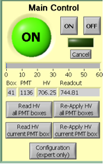
The HV on PMTs is usually ON during the Run. The two buttons on top are for turning the HV On and OFF on all PMT boxes. The most frequently used button on this subpanel is “Re-Apply HV all PMT Boxes” which is usually used to recover after HV trip. Sometimes you will need to “Re-Apply HV current PMT box” if the system does not set the HV on all boxes cleanly.
The scale 0-60 shows you a progress report. The small icons below this scale tells you what PMT box and PMT were addressed or readout.
Once you recover from a HV trip please pay attention to the small boxes labeled “Box”, “PMT”, and the speed at which the program reads the voltages on the PMTs. This will tell you which box has “Timeout” problems and which power supply will need to be power cycled.
Subpanel “PMTs In a Selected Box”
This subpanel shows you the status of the PMTs in a given PMT box.
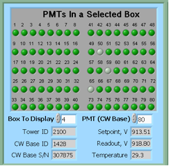
If you want to manually bring a single PMT box to the operational state by clicking on “Re-Apply HV current PMT box” on the Main Control subpanel you will need to specify which Box To Display on the panel first.
Subpanel “Alarm Control”
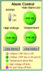
On the Alarm Control sub-panel the SOUND should be always ON, except for the case when you are recovering from a HV trip and wish to mute this annoying sound.
Shift personnel are asked to report HV trips in the shift log (type of trip, e.g. single box#, with or without timeout, massive trip, etc…)
Please don’t forget to switch this button back to the ON position after recovering from a trip.
The Main Alarm LED will switch color from green to red in case of an alarm.
HV trip with Timeout problem.
Typical situation – you hear a sound alarm indicating a HV trip. The auto-recovery program did not bring all PMT boxes to the operational state, e.g. some boxes will be shown in yellow. First thing to check for the presence of a “Timeout” problem.
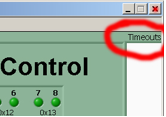
Look at the right upper corner of the GUI. If the field below “Timeouts” is blank then try to recover by re-applying HV to all PMT boxes if the number of bad boxes more then two. If only one or two boxes is yellow then you can try to re-apply HV to the current PMT box.
If only one or two PMT bases timed out and HV tripped try to recover using above procedure. It is possible that one or two PMT bases will timed without causing trips of HV, then just continue running and made a note in the shift log about timed out PMT bases, experts will take care of this problem during the day.
But it is also a chance that a single timed out PMT base will trip lots of other PMT. In this case this bad PMT should be masked out. The procedure to do this is simple and can be found at the end of this manual. However, this is an expert operation and should only be performed after consulting with a BEMC expert.
However, if the field below “Timeouts” is filled with numbers (these are PMTs addresses) then you have a Timeout problem. The procedure to recover is below:
- notify shift leader about this problem and tell him that it will take at least 20 min. to bring back BEMC for Physics running.
- Second, try to identify which PMT box has timeouts (usually it will be first box in yellow counting from 1 to 60). If you are not sure which box has the timeout problem then read all pmt boxes by clicking on corresponding button at the “Main Control” subpanel, and observe which box creates the problem. The box with timeout problem will be responding VERY slowly and will be clearly seen on the “Main Control” subpanel. At the same time, PMTs addresses will be appear in “Timeouts” white space to the right of the green control panel.
- As soon as you find the box with the timeout problem, click “Cancel” on the “Main Control” subpanel and then click “OFF” – you will need to turn HV OFF on all PMTs.
- Wait till HV is shut OFF (all PMT Boxes).
- From Terminal 1, power cycle correspondent PL512 (Off, wait 30 sec., On).
- Now turn ON HV on PMT boxes from the “Main Control” subpanel. It will take about 2 to 3 minutes first to send desired voltages to all PMTs and then read them back – if the HV is set correctly.
It is possible that during step (6) one of the BEMC PMT LV on the East or West side will trip. In this case cancel ramp (press “Cancel” button on the “Main Control” subpanel). Power cycle tripped BEMC PMT LV. Proceed with the slow ramp.
However, if during step (6) you still get a “Timeout” problem then you will need to:
- Call experts
-------------------- Changes for Run10 operation procedures ----------------------------
To reduce the number of HV trips and associated efficiency losses during data taking we changed functionality of the PMT HV program. Namely, the HV read back time interval was changed from 15 minutes to 9999 hours, because it was found that most of the HV trips were self induced during HV read back. As a result efficiency of data taking was improved for the price of “conscious operation”. You can‟t relay anymore on absence of the HV Trip alarm as an indicator that HV on all PMTs is at nominal values. Instead shift crew should monitor associated online plots during data taking to be sure that HV was not tripped. In particular, for Run 10, shift crew should watch two plots “ADC Eta Vs Phi” and “Tower ADC” under the “BEMC Shift” tab. Example of missed HV trip on one of the PMT box during recent data taking is shown below.
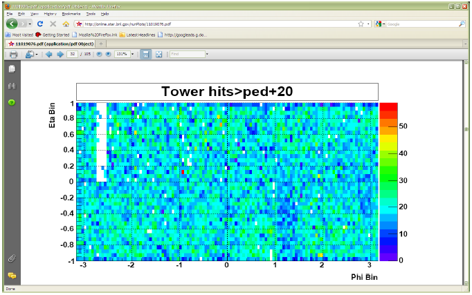
The white gap in the upper left corner shows absence of hits in BTOW due to HV trip in one of the BTOW PMT Box. It is easy to find out which box tripped by looking at second plot.
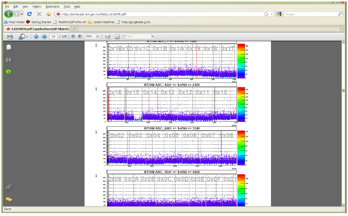
The gap with missing hits on the second subpanel for crate 0x15 will tell you that one of the PMT box 11 or 12 was tripped (correspondence between BTOW crates ID and PMT boxes is shown in the BTOW HV GUI see the picture at the beginning of this section).
What to do if shift crew will notify you of HV trip?
The fastest way to recover is to identify what box tripped and then try to recover only this PMT box. In some case it will be impossible to do this, because you will be needed to powercycle LV power supply for PMT HV system (timeout problems).
This is typical scenario:
1. Identify which PMT box(es) potentially tripped. (In the example above one PMT box 11 or 12 lost HV) to do that:
1.1 From the BTOW HV GUI form subpanel “PMTs In a Selected Box” select needed box in the “Box To Display” window.
1.2 From the BTOW HV GUI form subpanel “Main Control” press “Read HV current PMT Box”. (In the example above, detector operator found that Box 11 was OK after reading HV, but Box 12 had timeout problems).
1.3 Depending what will be result of (1.2) you may need to simply Re-Apply HV to current PMT box (no timeouts during step (1.2), or you will need to resolve timeout problem.
There are additional duties for detector operators when STAR is not taking data for long period of time for any reasons. We need to keep HV On on all PMTs at all time. This will assure stable gains on PMTs. If for some reasons PMTs will be Off for long time (few hours) then it will be difficult to assure that the PMTs gain will not drift once we turn HV On again. Typical situation is APEX days, when STAR is not taking data for 12 hours or so. To check that HV is on shift will be asked to take a short run 1k events using “bemcHTtest” configuration. TRG+DAQ+BTOW only. Once the data will be taken use a link from the run log browser to “LO Trigger”. Check page 6.
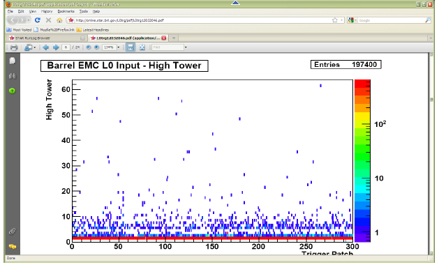
All trigger patches should have some hits. In case of the HV trips you will see blank spots.
Procedure to mask out single timeout PMT base.
Information you will need:
1. In which PMT box timeout PMT base is located
2. PMT (CW Base) to masked out.
In the timeout window the displayed number is CW Base ID this number need to be translated to PMT (CW Base).
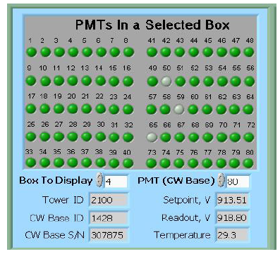
From this sub panel you can find out which PMT in the affected PMT box need to be masked out. Scroll thru the
PMT (CW Base) top right small window and read out at the same time CW Base ID in the second from the bottom left window. (As shown, PMT (CW Base) 80 correspond to CW Base ID 1428).
Now, click “Configuration (expert only)” button on the Main Control panel.
Another panel EMC_Configuration.vi will open.
From this panel click “CW Bases Configuration” button on the right bottom.
Another panel EMC_CWBasesConf.vi will open.
On this panel specify PMT BOX Number and then click on desired CW Base to be masked out. The color of the dot will change from bright green to pale green. Then click OK button.
Panel will close after that.
Click OK button on EMC_Configuration.vi panel, this panle will close after that.
To check that you masked out right CW Base, Re-Apply HV to current PMT box. Once HV will be re-applied you will see masked CW base will be in the gray color as shown in the picture above (Bases 50, 59, 65 were masked out in the PMT box 4).
Terminal 3. “BSMD HV Control”
Your login name is emc, your password is __________________________
This screenshot shows how the window on the terminal3 will look when the HV is Off on the BSMD modules. There should be two open windows. One is a LabView GUI and another is a telnet session SY1527 (CAEN HV Main Frame).
In normal operation it is a one click procedure to turn the HV On or OFF on the BSMD.
There is complete description of the BSMD HV program in a separate folder in this document.
Although, operation is very simple, attention should be made for audio alarms.
Do not mute the ALARM. Shift personnel are asked to report all BSMD trips in the shift log.
Terminal 0. “BPSD HV Control”
The BPSD (Barrel PreShower Detector) HV supplies are two Lecroy 1440 HV systems located on the second floor platform, racks 2C5. Each 1440 is commanded by a 1445A controller which communicates via the telnet server on the second floor of the platform (SCSERV [130.199.60.167]). The left supply uses port 9041 and the right supply uses port 9043.
The HV for BPRS should be On at all times.
From Run 10 for BPRS control we will be using new GUI. They will be open on one of the desktop on Terminal 0 (Beatrice.starp.bnl.gov). Usually detector operators no need to take any actions regarding BPRS HV unless specifically requested by experts. The screen shots of of the new GUIs shown below.
To start the GUI use type bemc_lecroy and bemc_lecroy2.


A Green LED indicators tells you that HV is On and at desired level.
You can open subpanel for any slot to read actual values of HV. The screen shot is shown below.

Please Ignore empty current charts – it is normal.
Sometime, BEMC PSD GUI can turn white, due to intermittent problems with LeCroy crate controller. Simply make a log in the shift log and continue normal operation. It is likely HV is still On and at desired level. Experts not need to be called right away in this case.
Easy Troubles:
BEMC Main Control seems to be frozen, e.g. program doesn’t respond to operators requests.
Probable reason: RadStone cards in a “funny state” and needs to be reset
From Terminal 1 try to:
- kill_emc
- soft reboot first “Ctrl” + “x” from HDLC terminal window.
- start emc and see if problem solved
If the problem is still there then:
- kill_emc
- Power Cycle Crate 80
- start emc and see if problem solved
If problem is still there call experts
PL512 Information (Run 11 configuration)
There are two PL512 power supplies which provides power to the BEMC PMT boxes. Both are located in the rack 2C2, second floor.
The top unit (IP address 130.199.60.79) serves West side of the detector. The bottom unit (IP address 130.199.60.81) serves East side of the detector. The connection scheme is shown below
PMT Boxes
West Side East Side
| 1-8 | 9-16 | 17-22 | 23-30 | 32-39 | 40-47 | 48-53 | 54-31 | |
| U 0,4,8 | 1,5,9 | 3,7,11 | 2,6,10 | 0,4,8 | 1,5,9 | 3,7,11 | 2,6,10 | |
| U 0,1,2,3 | +5 V | |||||||
| U 4,5,6,7 | -5 V | |||||||
| U 8,9,10,11 | +12 V |
Note , BEMC PMT Low Voltage Power Supply Slow Control channels enumerated from 1 to 12 in the Labview GUI.
Slow control for PL512 runs on EMC02, login as emc, alias PMT_LV.
You will need to specify IP address.
Configuration (Experts Only) password is ____________.
Log files will be created each time you will start PMT_LV in the directory
/home/emc/logs/
for example
/home/emc/logs/0703121259.txt (March 12, 2007, 12:59)
To restart PL512 epics applications.
Login to softioc1.starp.bnl.gov bemc/star_daq_sc
Look at procIDs
->screen –list
->screen –r xxxx.Bemc-west(east) xxxx is procID
->bemclvps2 > (ctrl A) to detach
exit to kill
->BEMC-West or East to restart
Experts control for PL512
If you need to adjust LV on PL512 you can do this using expert_bemc_west or (east).
These GUI has experts panel. Adjusting LV setting DO NOT try to slide the bars.
Instead click on it then on popup window you can simply type desired value.
Make sure you will close expert GUI and return to normal operational GUI once
you will finish adjustments.
A copy of this manual as a PDF document is available for download below.
Expert Contacts
Steve Trentalange (on site all run) e-mail: trent@physics.ucla.eduPhone: x1038 (BNL) or (323) 610-4724 (cell)
Oleg Tsai (on site all run) e-mail: tsai@physics.ucla.edu
Phone: x1038 (BNL)
SMD High Voltage Operation
Version 1.10 -- 04/25/06, O.D.TsaiOverview
The SMD detectors are a set of 120 proportional wire chambers located inside the EMC modules (one per module). The operating gas is Ar/CO2(90/10). The nominal operating voltage is +1430 V. As for any other gaseous detector, manipulation with high voltage should be performed with great care.A detailed description of the system is given in the Appendix.
SMD HV must be turned OFF before magnet ramp !
Standard Operation includes three steps.
Turn HV ON
Turn HV OFF
Log Defective Modules
To turn SMD HV ON the procedure is:
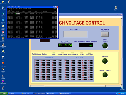
- On HOOSIER.STARP.BNL.GOV computer double click on the SMDHV icon on the Windows desktop. The 'SMD HIGH VOLTAGE CONTROL' window will open.
- On the SMD HIGH VOLTAGE CONTROL window click 'POWER' button.
- 'POWER' button will turn RED
- In no later than 90 + 150 + 300 sec in window 'Current Mode' you will see the message - "Physics Mode"
- All modules with high voltage on them will be shown in GREEN, LIGHT BROWN or YELLOW.
To turn HV OFF on SMD the procedure is:
- Click on the green 'POWER' button. Result:
- 'POWER' button will turn from green to BROWN
- after a 30 sec. or so small window will pop-up telling you that voltages an all channels reached zero.
- Click 'OK' on that small window to stop the program.
To Log Defective Modules
- Scroll down the window -- you will see three tables
- Log contents of the left table called 'Defect Module List' if any modules are presented here.
- Log contents of the right table called 'Modules tripped during Standby' (for example Run XXX #8 - 3 trips, Run XXX #54 - 1 trip)
- Close the 'SMD HIGH VOLTAGE CONTROL' window.
Detailed description of the SMD HV Program and associated hardware settings can be found in Appendix.
-------------------
Indicators to watch:
1. Interlock went RED
In case STAR global interlock went ON
- Interlock led will turn in RED
- the SMD HV program will turn OFF HV on all SMD channels and program will halt.
- Operator should close SMD HV Voltage control window.
Once STAR global interlock will be cleared follow usual procedure to power up SMD.
2. Server Timeout went RED or SMD HV Control program is frozen.
This is an unusual situation and SMD Expert Contacts should be alerted. The lost communication to SY1527 should not lead to immediate damages to the SMD chambers.
In case communication to the SY1527 is lost for some reason the 'SERVER TIMEOUT' led will turn RED. In case SMD HV Control program is frozen the 'Current Time' will not be updated.
Procedure to resolve problem is:
- Open terminal window on EMC01.STARP.BNL.GOV (monitor is on top of SMD HV Control PC)
- ping 130.199.60.50 -- observe that packets transmitted and received.
- If there are no communication with SY1527 (packets lost) -- Call one of the Expert Contacts!
- If communication is OK, then stop ping and type telnet 130.199.60.50 1527 -- You should see 'login window for CAEN SY1527 system'
- Press any key
- Login as 'admin' with password 'admin' -- you will see Main Menu window for SY1527
- From 'Main' chose 'Channels' by pressing 'Enter' -- you will see Channels menu window
- Verify HV is presented on channels (VMon)
Usually second terminal window is open on HOOSIER.STARP.BNL.GOV to monitor SY1527 HV power supply. If this window is not open use “putty” and open SY1527 session.
Now you can operate HV using this window, but if there is no emergency to turn HV OFF you should first try to restart SMD HV Control program.
Basic operations from that window are:
Turn HV OFF
Turn HV ON
Turn HV OFF
- press Tab key
- scroll to 'Groups' menu
- press 'Enter' to chose "Group Mode" --you will see highlighted column
- scroll to "Pw"
- press space bar -- you will see "Pw" will switched from On to Off and VMon will start to decrease.
- press Tab key
- select 'Group' mode
- scroll to IOSet
- type 5.0 (Current limit 5uA)
- scroll to Trip
- type 0.5 sec
- Verify that V0Set is 1430 V
- Scroll to Pw
- press Space bar -- you will see Pw will switch from OFF to ON and Status goes to Up. VMon will start to increase.
- Press Tab key
- reselect 'Group' mode
- Change I0Set and Trip for tripped channels
- Power them up - scroll to Pw, and press Space bar.
Appendix
Before you start:
"Be afraid, even paranoid, and that gives you a chance to catch bad effects in the early stages when they still do not matter"
--J. Va'vra (Wire Aging Conference)
Detailed information regarding SY1527 mainframe and A1733 HV distribution boards can be found at CAEN web page.
The SMD HV is supplied by the CAEN SY1527 HV system. The mainframe is located in rack 2C5 (Second Floor, Third Row, near the center). The HV cables run from modules to the SMD crates (15 cables per each crate). At each crate HV cables re-grounded on patch panels assuring same ground for HV and signals to be read. From SMD crates, the HV lines then run to the SY1527 system. There are 10 HV cards, 12 HV channels each (model A1733) inside the mainframe to supply high voltages to the SMD chambers. The parameters of the high voltage system controlled via Ethernet. The GUI based on LabView and CAEN OPC server.
Hardware settings are:
HV Hardware limit set to +1500 V on each of A1733 cards.
HV Software limit (SVMax) set to +1450 V for each channel.
Communications settings for SY1527 are:
IP           130.199.60.50
Net Mask     255.255.254.0
Gateway      0.0.0.0
User name    Admin
Password Admin(from top to bottom, HV is Off)
LED
Chk Pass On
Toggle Switch 'Loc enable' On
Ch Status 'NIM' On
Interlock 'Open'
Master On
+48 V On
+5 V On
+12 V On
-12 V On
Main On
Each A1733 card should have 50 Ohm Lemo 00 terminator to enable HV.
Description of SMD High Voltage Control program.
All SMD HV software is installed on EMCSC.STARP.BNL.GOV in folder C:/SY1527
The SMD HV Control provides one button operation of the HV system for the SMD. There are three main functions Power On, Physics Mode, Power Off. There are two configuration files Conf.txt and Conf2.txt which defines ramp up speed and trip settings for different mode of operation.
The nominal settings for Power On are (C:/SY1527/Conf.txt):
V0 1430 V
I0Set 5 uA
Trip 0.5 s
Ramp Down 50 V/sec
Ramp Up 20 V/sec
All channels are allowed to be ramp up in three consecutive attempts. If the first attempt (90 sec) for given channel lead to trip then ramp up speed will be set to 10 V/sec and second attempt (150 sec) will be performed. If second attempt will lead to trip then ramp up speed will be set to 7 V/sec and third attempt (300 sec) will be made. If all three attempt led to trip the program disconnect that particular channel from HV (corresponding led on main panel will turn in RED).
In no later then 90 + 150 + 300 seconds program will change parameters of I0Set and Trip form 5 uA and 0.5 sec to 1.6 uA and 0.1 sec and will switch to the Physics Mode.
The nominal settings for Physics Mode are (C:/SY1527/Conf2.txt)
V0 1430 V
I0Set 1.6 uA
Trip 0.1 s
Ramp Down 50 V/sec
Ramp Up 20 V/sec
Channels allowed to trip no more then 6 times during the Physics Mode. If channel will trip then I0Set and Trip for that particular channel will be set to 5 uA and 0.5 sec and program will try to bring that channel up. On front panel Alarm Status will turn in RED, corresponded message will pop up in 'Current Mode' window, and corresponded to that channel LED will turn in YELLOW or RED. Once voltage reach 90% of nominal all indicators will turn to normal status. Usually it takes about 15 seconds to bring channel back to normal. At the bottom of the screen the right table with modules that tripped during the Physics Mode will be updated. If some channel will trip more than 6 times that channel will be HV disabled by the program and corresponded led will turn RED. The left table on the bottom of the screen will be updated. Such cases should be treated by experts only later on.
All SMD channels during the Physics Mode is under the monitoring. Each 3 seconds or so, the values of Voltage, Current and time are logged in files XX_YY_ZZ_P.txt in C:/SY1527/Log, where XX - current month, YY - current day, ZZ - current year, and P is V for Voltages and I for Currents. The current time saved in seconds. The macro C:/SY1527/smdhv.C plots bad channels history and fills histograms for all other channels.
Turn Off is trivial and no need explanations.
The meaning of the LED on main panel are:
Green – channel is at nominal HV, current < 1 uA
Brown – channel is at nominal HV, 1 uA < current < 5 uA
Yellow – the HV is < 50% of nominal
Red - channel was disconnected due trips during ramp up or physics modes.
Black - channel disabled by user (Conf.txt, Conf2.txt)
It is important to monitor channels with high current (“Brown”), as well as channels that shows high number of trips during the operation. Note: some channels (54 for example) probably has a leakage on external HV distribution board and believed to be OK in terms of discharges on anode wires as was verified during summer shutdown. The other might develop sparking during the run or might have intermittent problems (#8 for example). If problems with sparking will be detected at early stages then those channels might be cured by experts during the run, without of loss of entire chamber as it was happened during the first two years of operation.
The C:/SY1527/ReadSingleChannel.vi allows to monitor single channel. You may overwrite nominal parameters of HV for any channel using that program (it is not desired to do that). This program can run in parallel with the Main SMD HV Control program. The operation is trivial, specify 'Channel to monitor' and click on 'Update Channel'. If you wish to overwrite some parameters (see above) then fill properly VOSet etc. icons and click on Update Write.
Important! Known bug. Before you start you better to fill all parameters, if you do not do that and stop the program later on the parameters will be overwritten with whatever it was in those windows, i.e. if V0Set was 0 then you will power Off the channel.
In some cases it is easy to monitor channels by looking at front panel of the SY1527 mainframe. The image of this panel can be
obtained by opening telnet session (telnet 130.199.60.50 1527) on EMC01.STARP.BNL.GOV.
All three programs can run in parallel.
-----Experts to be called day or night no matter what---
1. The operation crew lost communication with SY1527
2. Any accidental cases (large number (>5) of SMD channels
suddenly disconnected from HV during the run)
For experts only!
What to do with bad modules?
1. If anode wire were found broken then disable channel by changing 1430 to 0 in both configuration files. That should help to avoid confusions of detector operators.
2. If anode wires are OK, and module trips frequently during first half an hour after power Up then it is advised to set HV on that particular channel to lower value (-100V, -200V from nominal etc…) and observe the behavior of the chamber (ReadSingleChannel.vi). In some cases after a few hours module can be bring back to normal operation.
3. If step 2 did not help, then wait till scheduled access and try to cure chamber by applying reverse polarity HV. Important, you can do that using good HV power supply (fast trip protection, with current limit 5uA), or by using something like ‘Bertran’ with external microammeter and balance resistor of no less then 10 MOhm, only! In any case you need to observe the current while gradually increase HV. In no case ‘Bertarn’ like power supply might be left unattended during the cure procedure. It is not advised to apply more then -1000 V. In some cases curing procedure might be fast (one hour or so). In others it might take much longer (24 hours and more) to bring module back to operation. In any case I would request to talk with me.
4. The SMDHV is also installed on EMCSC.STARP.BNL.GOV and can be run from there, although that will for sure affect BTOW HV, be advised.
LOG:
Version 1.00 was written 11/12/03
Version 1.10 corrected 04/25/06
A copy of this manual as a Word document is available for download below.
Calibrations
Here you'll find links to calibration studies for the BEMC:
BTOW
2006
procedure used to set the HV online
MIP study to check HV values -- note: offline calibrations available at Run 6 BTOW Calibration
2005
final offline
2004
final offline
2003
offline slope calibration
MIPs
electrons
BSMD
2004
Dmitry & Julia - SMD correlation with BTOW for 200 GeV AuAu
BPSD
2005
Rory - CuCu PSD calibration studies
2004
Jaro - first look at PSD MIP calibration for AuAu data
BPRS
This task has been picked up by Rory Clarke from TAMU. His page is here:
Run 8 BPRS Calibration
Parent for Run 8 BPRS Calibration done mostly by Jan
01 DB peds R9069005, 9067013
Pedestal residua for 434 zero-bias events from run 9069005.
The same pedestal for all caps was used - as implemented in the offline DB.
Fig 1.

Fig 2. Run 9067013, excluded caps >120. All 4800 tiles, pedestal residua from 100 st_zeroBias events. Y-axis [-50,+150].

Fig 3. Run 9067013, excluded caps >120. Pedestal corrected spectra for all 4800 tiles, 10K st_physics events. Y-axis [-50,+150].
Dead MAPMT results with 4 patches 4 towers wide.

Fig 4.
Run 9067013, excluded caps >120.
Zoom-in Pedestal corrected spectra, one ped per channel.
Top 10K st_physics events (barrel often triggered)
Bottom pedestal residua 100 st_zeroBias events

Fig 5.
Run 9067013, input =100 events, accept if capID=124 , raw spectra.
There are 4 BPRS crates, so 1200 channels/crate. In terms of softIds it's
PSD1W: 1-300 + 1501-2400
PSD19W: 301-1500
PSD1E: 2401-2900 + 4101-4800
PSD20E: 2901-4100
Why only 2 channels fired in crate PSD20E ?

02 pedestal(capID)
Run 9067013, 30K st_physics events, spectra accumulated separately for every cap.
Top plot pedestal (channel), bottom plot integral of pedestal peak to total spectrum.
Fig 1. CAP=122

Fig 2. CAP=123

Fig 3. CAP=124

Fig 4. CAP=125

Fig 5. CAP=126

Fig 6. CAP=127

Fig 7. Raw spectra for capID=125. Left: typical good pedestal, middle: very wide pedestal, right: stuck lower bit.
For run 9067013 I found: 7 tiles with ADC=0, ~47 tiles with wide ped, ~80 tiles with stuck lower bit.
Total ~130 bad BPRS tiles based on pedestal shape, TABLE w/ bad BPRS tiles

Fig 8. QA of pedestals, R9067013, capID=125. Below is 5 plots A,...,F all have BPRS soft ID on the X-axis.
A: raw spectra (scatter plot) + pedestal from the fit as black cross (with error).
B: my status table based on pedestal spectrum. 0=good, non-zero =sth bad.
C: chi2/DOF from fitting pedestal, values above 10. were flagged as bad
D: sigma of pedestal fit, values aove 2.7 were flagged as bad
E: integral of the found pedestal peak to the total # of entries. On average there was ~230 entries per channel.

Fig 9. BPRS pedestals for 'normal' caps=113,114,115 shown with different colors

Fig 10. BPRS pedestals for caps=100..127 and all softID , white means bad spectrum, typical stats of ~200 events per softID per cap

Fig 11. BPRS:" # of bad caps , only capID=100...127 were examined.

Fig 12. BPRS:" sig(ped)

Fig 13. BPRS:" examples of ped distribution for selected channels. Assuming for sing;e capID sig(ped)=1.5, the degradation of pedestal resolution if capID is not accounted for would be: sqrt(1.5^2 +0.5^2)=1.6 - perhaps it is not worth the effort on average. There still can be outliers.

03 tagging desynchronized capID
BPRS Polygraph detecting corrupted capIDs.
Goal: tag events with desynchronized CAP id, find correct cap ID
Method:
- build ped(capID, softID)
- pick one BPRS crate (19W)
- compute chi2/dof for series capID+/-2
- pick 'best' capID with smallest chi2/dof
- use pedestals for best capID for this crate for this event
- if best capID differs from nominal capID call this event 'desynchronized & fixed'
Input: 23K st_physics events from run 9067013.
For technical reason limited range of nominal capID=[122,126] was used, what reduces data sample to 4% ( 5/128=0.04).
Results:
Fig 1. ADC-ped(capID,softID) vs. softID for crate 1 (i.e. PSD19W) as is'. No capID corruption detection.

Fig 2. ADC-ped(capID,softID) with capID detection & correction enabled. The same events.
Note, all bands are gone - the capID fix works.
Right: ADC-ped spectra: Black: 594 uncorrupted events, red: 30 corrupted & fixed events.
The integral for ADC[10,70] are 2914 and 141 for good and fixed events, respectively.
141/2914=0.048; 30/594=0.051 - close enough to call it the same (within stats).

Fig 3. Auxiliary plots.
TOP left: chi/dof for all events. About 1100 channels is used out of 1200 in served by crate 1. Rejected are bad & outliers.
TOP right: change of chi2/dof for events with corrupted & fixed capID.
BOTTOM: frequency of capID for good & fixed events, respectively.

Conclusions:
- BPRS-Polygraph algo efficiently identifies and corrects BPRS for corrupted capID, could be adopted to used offline .
- there is no evidence ADC integration widow changes for BPRS data with corrupted capID.
Table 1.
shows capIDs for the 4 BPRS crates for subsequent events. Looks like for the same event cap IDs are strongly correlated, but different.
Conclusion: if we discard say capID=125, we will make hole of 1/4 of barrel , different in every event. This holds for BPRS & BSMD.
capID= 83:89:87:90: eve=134
capID= 1:4:11:3: eve=135
capID= 74:74:81:72: eve=136
capID= 108:110:116:110: eve=137
capID= 68:72:73:75: eve=138
capID= 58:55:65:64: eve=139
capID= 104:110:106:101: eve=140
capID= 9:6:8:15: eve=141
capID= 43:37:47:46: eve=142
capID= 120:126:118:122: eve=143
capID= 34:41:41:40: eve=144
capID= 3:0:126:2: eve=145
capID= 28:33:28:30: eve=146
capID= 72:64:70:62: eve=147
capID= 2:6:7:5: eve=148
capID= 22:32:33:24: eve=149
capID= 8:4:5:124: eve=150
capID= 23:17:17:19: eve=151
capID= 62:57:63:61: eve=152
capID= 54:53:45:47: eve=153
capID= 68:75:70:67: eve=154
capID= 73:79:73:72: eve=155
capID= 104:98:103:103: eve=156
capID= 12:5:13:10: eve=157
capID= 5:10:10:2: eve=158
capID= 32:33:27:22: eve=159
capID= 96:102:106:97: eve=160
capID= 79:77:72:77: eve=161
04 BPRS sees beam background?
The pair of plots below demonstrates BPRS pedestal residua are very clean once peds for 128 caps are used and this 5% capID corruption is detected and fixed event by event.
INPUT: run 9067013, st_phys events, stale BPRS data removed, all 38K events .
Fig 0. capID correction was enabled for the bottom plot. Soft ID is on the X-axis; rawAdc-ped(softID, capID) on the Y-axis.

Now you can believe me the BPRS pedestals are reasonable for this run. Look at the width of pedestal vs. softID, shown in Fig 1 below.
There are 2 regions with wider peds, marked by magenta(?) and red circle.
The individual spectra look fine (fig 2b, 2bb).
But the correlation of pedestal width with softID (fig 1a,1b) and phi-location of respective modules (fig 3a, 3b) suggest it could be due to the beam background at
~7 o'clock on the West and at 6-9 o'clock on the East.

05 ---- peds(softID,capID) & status table, ver=2.2, R9067013
INPUT: st_hysics events from run=9067013
Fig 1. Top: pedestal(softID & capID), middle: sigma of pedestal, bottom: status table, Y-axis counts how many capID had bad spectra.
Based on pedestal spectra there are 134 bad BPRS tiles.

Fig 2. Distribution of pedestals for 4 selected softIDs, one per crate.

Fig 3. Zoom-in of ped(soft,cap) spectrum to see there is more pairs of 2 capID which have high/low pedestal vs. average, similar to the known pair (124/125).
Looks like such piar like to repeat every 21 capIDs - is there a deeper meaning it?
(I mean will the World end in 21*pi days?)

Fig 4. Example of MIP spectra (bottom). MIP peak is very close to pedestal, there are worse cases than the one below. 
06 MIP algo ver 1.1
TPC based MIP algo was devised to calibrate BPRS tiles.
Details of the algo are in 1st PDF,
example of MIP spectra for 40 tails with ID [1461,1540] are in subsequent 5 PDF files, sorted by MAPMT
Fig 1 shows collapsed ADC-ped response for all 4800 BPRS tiles. The average MIP response is only 10 ADC counts above ped wich has sigma of 1.5 ADC. The average BPRS gain is very is very low. 
07 BPRS peds vs. time
Fig 1. Change of BPRS pedestal over ... within the same fill, see softID~1000
Pedestal residua (Y-axis) vs. softID (X-axis), same reference pedestals used from day 67 (so some peds are wrong for both runs) were used both plots.
Only fmsslow events, no further filtering, capID corruption fixed in fly.
Top run 9066001, start 0:11 am, fill 9989
Bottom run 9066012, start 2:02 am, fill 9989

Fig 2. Run list. system config was changed between those 2 runs marked in blue.

Fig 3. zoom in of run 9066001

Fig 4. another example of BPRS ped jump between runs: 9068022 & 9068032, both in the same fill.

08 BPRS ped calculation using average
Comparison of accuracy of pedestal calculation using Gauss fit & plain average of all data.
The plain average method is our current scheme for ZS for BPRS & BSMD for 2009 data taking.
Fig 2. TOP: RMS of the plain average, using 13K of fmsslow-triggered events which are reasonable surrogate of minBias data for BPRS.
Middle: sigma of pedestal fit using Gauss shape
Bottom: ratio of pedestals from this 2 method. The typical pedestal value is of 170 ADC. I could not make root to display the difference, sorry.

09 BPRS swaps, IGNORING Rory's finding from 2007, take 1
This page is kept only for the record- information here is obsolete.
This analysis does not accounts for BPRS swaps discovered by Rory's in 2007, default a2e maker did not worked properly
- INPUT: ~4 days of fmsslow-triggered events, days 65-69
- DATA CORRECTIONS:
- private BPRS peds(cap,softID) for every run,
- private status table, the same , based on one run from day 67
- event-by-event capID corruption detection and correction
- use vertex with min{|Z|}, ignore ranking to compensate for PPV problem
- TRACKING:
- select prim tracks with pr>0.4 GeV, dEdX in [1.5,3.7] keV, |eta|<1.2
- require track enters tower 1cm from the edge and exists tower at any distance to the edge
- tower ADC is NOT used (yet)
- 2 histograms of rawADC-ped were accumulated: for all events (top plot) and for BPRS tiles pointed by TPC track (middle plot w/ my mapping & lower plot with default mapping)
There are large section of 'miples' BPRS tiles if default mapping is used: 3x80 tiles + 2x40 tiles=320 tiles, plus there is a lot of small mapping problems. Plots below are divided according to 4 BPRS crates - I assumed the bulk of mapping problems should be contained within single crate.
Fig 1, crate=0, Middle plot is after swap - was cured for soft id [1861-1900]
   if(softID>=1861 && softID<=1880) softID+=20;
    else if(softID>=1881 && softID<=1900) softID-=20;

Fig2, crate=1, Middle plot is after swap - was cured for soft id [661-740]
  if(softID>=661 && softID<=700) softID+=40;
    else if(softID>=701 && softID<=740) softID-=40;

Fig3, crate=2, Middle plot is after swap - was cured for soft id [4181-4220].
But swap in [2821-2900] is not that trivial - suggestions are welcome?
 if(softID>=4181 && softID<=4220) softID+=40;
    else if(softID>=4221 && softID<=4260) softID-=40;

Fig4, crate=3, swap in [3781-3800] is not that trivial - suggestions are welcome?

10 -------- BPRS swaps take2, _AFTER_ applying Rory's swaps
2nd Correction of BPRS mapping (after Rory's corrections are applied).
- INPUT: ~7 days of fmsslow-triggered events, days 64-70, 120 runs
- DATA CORRECTIONS:
- private BPRS peds(cap,softID) for every run,
- private status table, excluded only 7 strips with ADC=0
- event-by-event capID corruption detection and correction
- use vertex with min{|Z|}, ignore PPV ranking, to compensate for PPV problem
- BPRS swaps detected by Rory in 2007 data have been applied
- TRACKING:
- select prim tracks with pr>0.4 GeV, dEdX in [1.5,3.7] keV, |eta|<1.2, zVertex <50 cm
- require track enters tower 1cm from the edge and exist the same tower at any distance to the edge (0 cm)
- tower ADC is NOT used (yet)
- 3 2D histograms of were accumulated:
- rawADC-ped (softID) for all events
- the same but only for BPRS tiles pointed by QAed MIP TPC track
- frequency of correlation BPRS tiles with MIP-like ADC=[7,30] with towers pointed by TPC MIP track
Based on correlation plot (shown as attachment 6) I found ~230 miss-mapped BPRS tiles (after Rory's correction were applied).
Once additional swaps were added ( listed in table 1, and in more logical for in attachment 3) the correlation plot is almost diagonal, shown in attachment 1.
Few examples of discovered swaps are in fig1. The most important are 2 series of 80 strips, each shifted by 1 software ID.
Fig 2 shows MIP signal shows up after shit by 1 softID is implemented.
The ADC spectra for all 4800 strips are shown in attachment 2. Attachment 5 & 6 list basic QA of 4800 BRS tiles for 2 cases: only Rory's swaps and Rory+Jan swaps.
Fig 1. Examples of swaps, dotted line marks the diagonal. Vertical axis shows towers pointed by TPC MIP track. X-axis shows BPRS soft ID if given ADC was in the range [7,30] - the expected MIP response. Every BPRS tile was examined for every track, multiple times per event if more than 1 MIP track was found.
Left: 4 sets of 4 strips needs to be rotated. Right: shift by 1 of 80 strips overlaps with rotation of 6 strips.

Fig 2. Example of recovered 80 tiles for softID~2850-2900. Fix: softID was shifted by 1.

Fig 3. Summary of proposed here corrections to existing BPRS mapping

Table 1. List of all BPRS swaps , ver 1.0, found after Rory's corrections were applied, based on 2008 pp data from days 64-70.
The same list in human readable from is here
Identified BPRS 233 swaps. Convention: old_softID --> new_softID
389 --> 412 , 390 --> 411 , 391 --> 410 , 392 --> 409 , 409 --> 392 ,
 410 --> 391 , 411 --> 390 , 412 --> 389 , 681 --> 682 , 682 --> 681 ,
 685 --> 686 , 686 --> 685 ,1074 -->1094 ,1094 -->1074 ,1200 -->1240 ,
1220 -->1200 ,1240 -->1260 ,1260 -->1220 ,1301 -->1321 ,1303 -->1323 ,
1313 -->1333 ,1321 -->1301 ,1323 -->1303 ,1333 -->1313 ,1878 -->1879 ,
1879 -->1878 ,1898 -->1899 ,1899 -->1898 ,2199 -->2200 ,2200 -->2199 ,
2308 -->2326 ,2326 -->2308 ,2639 -->2640 ,2640 -->2639 ,2773 -->2793 ,
2793 -->2773 ,2821 -->2900 ,2822 -->2821 ,2823 -->2822 ,2824 -->2823 ,
2825 -->2824 ,2826 -->2825 ,2827 -->2826 ,2828 -->2827 ,2829 -->2828 ,
2830 -->2829 ,2831 -->2830 ,2832 -->2831 ,2833 -->2832 ,2834 -->2833 ,
2835 -->2834 ,2836 -->2835 ,2837 -->2836 ,2838 -->2837 ,2839 -->2838 ,
2840 -->2839 ,2841 -->2840 ,2842 -->2841 ,2843 -->2842 ,2844 -->2843 ,
2845 -->2844 ,2846 -->2845 ,2847 -->2846 ,2848 -->2847 ,2849 -->2848 ,
2850 -->2849 ,2851 -->2850 ,2852 -->2851 ,2853 -->2852 ,2854 -->2853 ,
2855 -->2854 ,2856 -->2855 ,2857 -->2856 ,2858 -->2857 ,2859 -->2858 ,
2860 -->2859 ,2861 -->2860 ,2862 -->2861 ,2863 -->2862 ,2864 -->2863 ,
2865 -->2864 ,2866 -->2865 ,2867 -->2866 ,2868 -->2867 ,2869 -->2868 ,
2870 -->2869 ,2871 -->2870 ,2872 -->2871 ,2873 -->2872 ,2874 -->2873 ,
2875 -->2874 ,2876 -->2875 ,2877 -->2876 ,2878 -->2877 ,2879 -->2878 ,
2880 -->2879 ,2881 -->2880 ,2882 -->2881 ,2883 -->2882 ,2884 -->2883 ,
2885 -->2884 ,2886 -->2885 ,2887 -->2886 ,2888 -->2887 ,2889 -->2888 ,
2890 -->2889 ,2891 -->2890 ,2892 -->2891 ,2893 -->2892 ,2894 -->2893 ,
2895 -->2894 ,2896 -->2895 ,2897 -->2896 ,2898 -->2897 ,2899 -->2898 ,
2900 -->2899 ,3121 -->3141 ,3141 -->3121 ,3309 -->3310 ,3310 -->3309 ,
3717 -->3777 ,3718 -->3778 ,3719 -->3779 ,3720 -->3780 ,3737 -->3757 ,
3738 -->3758 ,3739 -->3759 ,3740 -->3760 ,3757 -->3717 ,3758 -->3718 ,
3759 -->3719 ,3760 -->3720 ,3777 -->3737 ,3778 -->3738 ,3779 -->3739 ,
3780 -->3740 ,3781 -->3861 ,3782 -->3781 ,3783 -->3782 ,3784 -->3783 ,
3785 -->3784 ,3786 -->3785 ,3787 -->3786 ,3788 -->3787 ,3789 -->3788 ,
3790 -->3789 ,3791 -->3790 ,3792 -->3791 ,3793 -->3792 ,3794 -->3793 ,
3795 -->3794 ,3796 -->3835 ,3797 -->3836 ,3798 -->3797 ,3799 -->3798 ,
3800 -->3799 ,3801 -->3840 ,3802 -->3801 ,3803 -->3802 ,3804 -->3803 ,
3805 -->3804 ,3806 -->3805 ,3807 -->3806 ,3808 -->3807 ,3809 -->3808 ,
3810 -->3809 ,3811 -->3810 ,3812 -->3811 ,3813 -->3812 ,3814 -->3813 ,
3815 -->3814 ,3816 -->3855 ,3817 -->3856 ,3818 -->3817 ,3819 -->3818 ,
3820 -->3819 ,3821 -->3860 ,3822 -->3821 ,3823 -->3822 ,3824 -->3823 ,
3825 -->3824 ,3826 -->3825 ,3827 -->3826 ,3828 -->3827 ,3829 -->3828 ,
3830 -->3829 ,3831 -->3830 ,3832 -->3831 ,3833 -->3832 ,3834 -->3833 ,
3835 -->3834 ,3836 -->3795 ,3837 -->3796 ,3838 -->3837 ,3839 -->3838 ,
3840 -->3839 ,3841 -->3800 ,3842 -->3841 ,3843 -->3842 ,3844 -->3843 ,
3845 -->3844 ,3846 -->3845 ,3847 -->3846 ,3848 -->3847 ,3849 -->3848 ,
3850 -->3849 ,3851 -->3850 ,3852 -->3851 ,3853 -->3852 ,3854 -->3853 ,
3855 -->3854 ,3856 -->3815 ,3857 -->3816 ,3858 -->3857 ,3859 -->3858 ,
3860 -->3859 ,3861 -->3820 ,4015 -->4055 ,4016 -->4056 ,4017 -->4057 ,
4018 -->4058 ,4055 -->4015 ,4056 -->4016 ,4057 -->4017 ,4058 -->4018 ,
4545 -->4565 ,4546 -->4566 ,4549 -->4569 ,4550 -->4570 ,4565 -->4545 ,
4566 -->4546 ,4569 -->4549 ,4570 -->4550 ,
For the reference:
- mapping of BPRS softID to MAPMT made by Will J. in 2007 is shown here: http://www.star.bnl.gov/protected/emc/wwjacobs/tmp/bprs_tubehookup_run7.pdf
Identified BPRS hardware problems:

Tiles w/ ADC=0 for all events:

* 3301-4, 3322-4 - all belong to PMB44-pmt1, dead Fee in 2007
   belonging to the same pmt:
     3321 has pedestal only
     3305-8 and 33205-8  have nice MIP peaks, work well

* 2821, 3781 , both at the end of 80-chanel shift in mapping
     neighbours of 2821: 2822,... have nice MIP
     similar for neighbours of 3781

* 4525, 4526 FOUND! should be readout from cr=2 position 487 & 507, respectively

I suspect all those case we are reading wrong 'positon' from the DAQ file


Pair of consecutive tiles with close 100% cross talk, see Fig 4.
35+6, 555+6, 655+6, 759+60, 1131+2, 1375+6, 1557+8,
2063+4, 2163+4, 2749+50, 3657+8,
3739 & 3740 copy value of 3738 - similar case but with 3 channels.
4174+5


Hot pixels, fire at random
1514, 1533, 1557,
block: 3621-32, 3635,3641-52 have broken fee, possible mapping problem
block: 3941-3976 have broken fee


Almost copy-cat total 21 strips in sections of 12+8+1
3021..32, 3041..48, 3052
All have very bread pedestal. 3052 may show MIP peak if its gain is low.
Fig 4. Example of pairs of correlated channels.

11 BPRS absolute gains from MIP, ver1.0 ( example of towers)
BPRS absolute gains from MIP, ver 1.0
Fig 1 Typical MIP signal seen by BPRS(left) & BTOW (right) for soft ID=??, BPM16.2.x (see attachment 1 for more)
Magenta line is at MIP MPV-1*sigma -> 15% false positives

Fig 2 Typical MIP signal seen by BPRS, pmt=BPM16.2
Average gain of this PMT is on the top left plot, MIP is seen in ADC=4.9, sig=2.6

Fig 3 Most desired MIP signal (ADC=16) seen by BPRS(left) & BTOW (right) for soft ID=1388, BPM12.1.8
Magenta line is at MIP MPV-1*sigma -> 15% false positives, (see attachment 2 for more)

Fig 4 Reasonable BPRS, pmt=BPM11.3, pixel to pixel gain variations is small

Fig 5 High MIP signal (ADC=28) seen by BPRS(left) & BTOW (right) , BPM11.5.14
Magenta line is at MIP MPV-1*sigma -> 15% false positives, (see attachment 3 for more)

Fig 6 High gain BPRS, pmt=BPM11.5

12 MIP gains ver1.0 (all tiles, also BTOW)
This is still work in progress, same algo as on previous post.
Now I run on 12M events (was 6 M) and do rudimentary QA on MIP spectra, which results with ~10% channel loss (the bottom figure). However, the average MIP response per tile is close to the final value.
Conclusion: only green & light yellow tiles have reasonable MIP response of ~15 ADC. For blue we need to rise HV, for red we can lower it (to reduce after pulsing). White area are masked/dead pixels.
Fig 1: BPRS MIP gains= gauss fit to MIP peak.
A) gains vs. eta & phi to see BPM pattern. B) gains with errors vs. softID, C) sigma MIP shape, D) tiles killed in QA

Fig 2: BTOW MIP gains= gauss fit to MIP peak. Content of this plot may change in next iteration.
A) gains vs. eta & phi. "ideal" MIP is at ADC=18, all towers. Yellow& red have significantly to high HV, light blue & blue have too low HV.
B) gains with errors vs. softID, C) sigma MIP shape, D) towers killed in QA

13 MIP algo, ver=1.1 (example of towers)
This is an illustration of improvement of MIP finding efficiency if ADC gates are set on BPRS & BTOW at the places matched to actual gains instead of fixed 'ideal' location.
Fig 1 is from previous iteration (item 11) with fixed location MIP gates. Note low MIP yield in BPRS (red histo) due to mismatched BTOW ADC gate (blue bar below green histo).

Fig 2 New iteration with adjusted MIP gates. (marked by blue dashed lines).
MIP ADC gate is defined (based on iteration 1) by mean value of the gauss fit +/- 1 sigma of the gauss width, but not lower than ADC=3.5 and not higher than 2* mean ADC
Note similar MIP yield in BPRS & BTOW. Also new MIP peak position from Gauss fit did not changed, meaning algo is robust. The 'ideal' MIP ADC range for BTOW is marked by magenta bar (bottom right) - is visibly too low.

Attached PDF shows similar plots for 16 towers. Have a look at page 7 & 14
14 ---- MIP gains ver=1.6 , 90% of 4800 tiles ----
BPRS absolute gains using TPC MIPs & BTOW MIP cut, ver 1.6 , 2008 pp data
- INPUT: fmsslow-triggered events, days 43-70, 525 runs, 16M events (see attachment 1)
- BTOW peds & ped-status from offline DB
- DATA CORRECTIONS (not avaliable using official STAR software)
- discard stale events
- private BPRS peds(cap,softID) for every run,
- private status table
- event-by-event capID corruption detection and correction
- use vertex with min{|Z|}, ignore PPV ranking, to compensate for PPV problem
- BPRS swaps detected by Rory in 2007 data have been applied
- additional ~240 BPRS swaps detected & applied
- BTOW ~50 swaps detected & applied
- BTOW MIP position determine independently (offline DB gains not used)
- TRACKING:
- select prim tracks with pr>0.35 GeV, dEdX in [1.5,3.3] keV, |eta|<1.3, zVertex <60 cm, last point on track Rxy>180cm
- require track enters & exits a tower 1cm from the edge, except for etaBin=20 - only 0.5cm is required (did not helped)
- triple MIP coincidence, requires the following (restrictive) cuts:
- to see BPRS MIP ADC : TPC MIP track and in the same BTOW tower ADC in MIP peak +/- 1 sigma , but above 5 ADC
- to see BTOW MIP ADC : TPC MIP track and in the same BPRS tile ADC in MIP peak +/- 1 sigma , but above 3.5 ADC
Fig 1. Example of typical BPRS & BTOW MIP peak determine in this analysis.
MIP ADC gate (blue vertical lines) is defined (based on iteration 1.0) by the mean value of the gauss fit +/- 1 sigma of the gauss width, but not lower than ADC=3.5 (BPRS) or 5 (BTOW) and not higher than 2* mean ADC.
FYI, the nominal MIP ADC range for BTOW (ADC=4096 @ ET=60 GeV/c) is marked by magenta bar (bottom right).
- Attachment 6 contains 4800 plots of BPRS & BTOW like this one below ( large 53MB !!)
- Numerical values of MIP peak position,width, yield for all 4800 BPRS tiles are in attachment 4.

Fig 2. ADC of MIP peak for 4800 BPRS tiles.
Top plot: mean, X-axis follows eta bin , first West then East. Y-axis follows |eta| bin, 20 is at physical eta=+/- 1.0.Large white areas are due to bad BPRS MAPMT (4x4 or 2x8 channels), single white rectangles are due to bad BPRS tile or bad BTOW tower.
Middle plot: mean +/- error of mean, X-axis =soft ID. One would wish mean MIP value is above 15 ADC to place MIP cut comfortable above the pedestal (sig=1.5-1.8 ADC counts).
Bottom plot: width of MIP distribution. Shows the width of MIP shape is comparable to the mean and we want to put MIP cut well below the mean to not loose half of discrimination power.
Note, the large # 452 of not calibrated BPRS tiles does not mean that many are broken. There are 14 known bad PMTs and e 'halves' , total=15*16=240 (see attachment 2). There rest are due broken towers (required by MIP coincidence) and isolated broken fibers, FEE channels.

Fig 3. Example of PMT with fully working 16 channels.
Top left plot shows average MIP ADC from 16 pixels. Top middle: correlation between MIP peak ADC and raw slope - can be used for relative gain change in 2009. Top right shows BTOW average MIP response.
Middle: MIP spectra for 16 pixels.
Bottom: raw spectra fro the same 16 pixels.
300 plots like this is in attachment 3.

Fig 4. Top plot: average over 16 pixels MIP ADC for 286 BPRS pmts. X axis = PMB# [1-30] + pmt #[1-5]/10. Error bars represent RMS of distribution (not error of the mean).
Middle plot : ID of 14 not calibrated PMTs. For detailed location of broken PMTs see attachment 2, the red computer-generated ovals on the top of 2007 Will's scribbles mark broken PMTs (blue ovals are repaired PMTs) found in this 2008 analysis.
Bottom plot shows # of pixels in given PMT with reasonable MIP signal (used in the top figure).
- Numerical values of MIP peak per PMT are in attachment 5.

Fig 5. ADC of MIP peak for 4800 BTOW tower. Top lot: mean, middle plot: mean +/- error of mean, bottom plot: width of MIP
- Numerical values of MIP peak position,width, yield for all 4800 BTOW towers are in attachment 4.
Note, probably 1/2 of not calibrated BTOW towers are broken, the other half is due to bad BPRS tiles, required to work by this particular algo.

Koniec !!!
15 Broken BPRS channels ver=1.6, based on data from March of 2008
The following BPRS pmts/tiles have been found broken or partially not functioning, based on reco MIP response from pp 2008 data.
Based on PMT-sorted spectra available HERE (300 pages , 3.6MB)
Table 1. Simply dead PMT's. Raw spectra contain 16 nice pedestals, no energy above, see Fig 2.
PMB,pmt, PDF page # , 16 mapped softIDs
2,3     8, 2185 2186 2187 2188 2205 2206 2207 2208 2225 2226 2227 2228 2245 2246 2247 2248
2,4,    9, 2189 2190 2191 2192 2209 2210 2211 2212 2229 2230 2231 2232 2249 2250 2251 2252
4,5,   20, 2033 2034 2035 2036 2053 2054 2055 2056 2073 2074 2075 2076 2093 2094 2095 2096
5,1,   21, 1957 1958 1959 1960 1977 1978 1979 1980 1997 1998 1999 2000 2017 2018 2019 2020
12,2,  57, 1421 1422 1423 1424 1425 1426 1427 1428 1441 1442 1443 1444 1445 1446 1447 1448
14,1,  66, 1221 1222 1223 1224 1225 1226 1227 1228 1241 1242 1243 1244 1245 1246 1247 1248
24,4, 119, 433 434 435 436 453 454 455 456 473 474 475 476 493 494 495 496
25,4, 124, 353 354 355 356 373 374 375 376 393 394 395 396 413 414 415 416
26,4, 129, 269 270 271 272 289 290 291 292 309 310 311 312 329 330 331 332
32,3, 158, 2409 2410 2411 2412 4749 4750 4751 4752 4769 4770 4771 4772 4789 4790 4791 4792
44,5, 220, 3317 3318 3319 3320 3337 3338 3339 3340 3357 3358 3359 3360 3377 3378 3379 3380
39,2, 192, 2905 2906 2907 2908 2925 2926 2927 2928 2945 2946 2947 2948 2965 2966 2967 2968
Table 2. FEE is broken (or 8-connector has a black tape), disabling 1/2 of PMT, see Fig 3.
PMB,pmt,  nUsedPix,  avrMIP (adc), rmsMIP (adc),PDF page # , all mapped softIDs
7,1,   7,   19.14, 4.36,  31, 1797 1798 1799 1800 1817 1818 1819 1820 1837 1838 1839 1840 1857 1858 1859 1860
40,1,  8,    5.16, 0.53, 196, 2981 2982 2983 2984 3001 3002 3003 3004 3021 3022 3023 3024 3041 3042 3043 3044
40,2,  6,    5.44, 0.80, 197, 2985 2986 2987 2988 3005 3006 3007 3008 3025 3026 3027 3028 3045 3046 3047 3048
40,3, 12,    8.50, 1.05, 198, 2989 2990 2991 2992 3009 3010 3011 3012 3029 3030 3031 3032 3049 3050 3051 3052
44,1, 10,   13.72, 8.24, 216, 3301 3302 3303 3304 3305 3306 3307 3308 3321 3322 3323 3324 3325 3326 3327 3328
45,2,  8,    5.04, 1.55, 222, 3421 3422 3423 3424 3425 3426 3427 3428 3441 3442 3443 3444 3445 3446 3447 3448
51,5,  7,   11.37, 2.15, 255, 3877 3878 3879 3880 3897 3898 3899 3900 3917 3918 3919 3920 3937 3938 3939 3940
52,5,  8,   15.84, 4.80, 260, 3957 3958 3959 3960 3977 3978 3979 3980 3997 3998 3999 4000 4017 4018 4019 4020
60,1,  8,   15.12, 3.41, 296, 4581 4582 4583 4584 4601 4602 4603 4604 4621 4622 4623 4624 4641 4642 4643 4644
Table 3. Very low yield of MIPs (1/5 of typical), may de due to badly sitting optical connector, see Fig 4
PMB,pmt, QAflag, nUsedPix,  avrMIP (adc), rmsMIP (adc),PDF page # , all mapped softIDs
10,5,  14,     0,  0.00, 0.00,  50, 1553 1554 1555 1556 1573 1574 1575 1576 1593 1594 1595 1596 1613 1614 1615 1616
31,5,  14,     0,  0.00, 0.00, 155, 4677 4678 4679 4680 4697 4698 4699 4700 4717 4718 4719 4720 4737 4738 4739 4740
37,2,   0,    10, 12.90, 7.41, 182, 2745 2746 2747 2748 2765 2766 2767 2768 2785 2786 2787 2788 2805 2806 2807 2808
49,1,   0,    16,  9.36, 3.55, 241, 3701 3702 3703 3704 3705 3706 3707 3708 3721 3722 3723 3724 3725 3726 3727 3728
Table 4. Stuck LSB in FEE, we can live with this. (do NOT mask those tiles)
PMB,pmt, QAflag, nUsedPix,  avrMIP (adc), rmsMIP (adc),PDF page # , all mapped softIDs
51,1,0, 15,   8.37, 1.30, 251, 3861 3862 3863 3864 3881 3882 3883 3884 3901 3902 3903 3904 3921 3922 3923 3924
51,2,0, 16,   8.66, 1.06, 252, 3865 3866 3867 3868 3885 3886 3887 3888 3905 3906 3907 3908 3925 3926 3927 3928
51,3,0, 16,  11.08, 1.28, 253, 3869 3870 3871 3872 3889 3890 3891 3892 3909 3910 3911 3912 3929 3930 3931 3932
51,4,0, 16,  17.16, 2.70, 254, 3873 3874 3875 3876 3893 3894 3895 3896 3913 3914 3915 3916 3933 3934 3935 3936
Table 5. Other problems:
PMB,pmt, QAflag, nUsedPix,  avrMIP (adc), rmsMIP (adc),PDF page # , all mapped softIDs
31,2,0, 16,  12.32, 3.73, 152,4665 4666 4667 4668 4685 4686 4687 4688 4705 4706 4707 4708 4725 4726 4727 4728
Fig 1. Example of fully functioning PMT (BPM=4, pmt=5). 16 softID are listed at the bottom o fthe X-axis.
Top plot: ADC spectra after MIP condition is imposed based on TPC track & BTOW response.
Bottom plot: raw ADC spectra for the same channels.

Fig 2. Example of dead PMT with functioning FEE.

Fig 3. Example of half-dead PMT, comes in pack, most likely broken FEE.

Fig 4. Example of weak raw ADC, perhaps optical connector got loose.

Fig 5. Example of stuck LSB, We can live with this, but gain hardware must be ~10% higher (ADC--> 18)

16 correlation of MIP ADC vs. raw slopes
Scott asked for crate based comparison of MIP peak position vs. raw slopes .
I selected 100 consecutive BPRS tiles, in 2 groups, from each of the 4 crates. The crate with systematic lower gain is the 4th (PSD-20E).
The same spectra from pp 2008 fmsslow events are used as for all items in the Drupal page.
Fig 1. BPRS carte=PSD-1W

Fig 2. BPRS carte=PSD-19W

Fig 3. BPRS carte=PSD-1E

Fig 4. BPRS carte=PSD-20E This one has lower MIP peak

Run 9 BPRS Calibration
Parent for Run 9 BPRS Calibration
01 BPRS live channels on day 82, pp 500 data
Status of BPRS live channels on March 23, 2009, pp 500 data.
Input: 32K events accepted by L2W algo, from 31 runs taken on day 81 & 82.
Top fig shows high energy region for 4800 BPRS tiles
Middle fig shows pedestal region, note we have ZS & ped subtracted data in daq - plots is consistent. White area are not functioning tiles.
Bottom fig: projection of all tiles. Bad channels included. Peak at ADC~190 is from corrupted channels softID~3720. Peak at the end comes most likely form saturation of BPRS if large energy is deposited. It is OK - BPRS main use is as a MIP counter.
Attached PDF contains more detailed spectra so one can see every tile.

BSMD
Collected here is information about BSMD Calibrations.
There are 36,000 BSMD channels, divided into 18,000 strips in eta and 18,000 strips in phi. They are located 5.6 radiation lengths deep in the Barrel Electromagnetic Calorimeter (BEMC).
1) DATA: 2008 BSMD Calibration
Information about the 2008 BSMD Calibration effort will be posted below as sub-pages.
Fig 1. BSMD-E 2D mapping of soft ID. (plot for reverse mapping is attached)

01) raw spectra
Goals:
- verify pedestals loaded to DB are reasonable for 2008 pp data
- estimate stats needed to find slopes of individual strips for minB events
Method:
- look at pedestal residua for individual strips, exclude caps 1 & 2, use only status==1
- fit gauss & compare with histo mean
- find integrals of individual strips, sum over 20 ADC channels starting from ped+5*sig
To obtain muDst w/o zero suppression I run privately the following production chain:
chain="DbV20080703 B2008a ITTF IAna ppOpt VFPPV l3onl emcDY2 fpd ftpc
trgd ZDCvtx NosvtIT NossdIT analysis Corr4 OSpaceZ2 OGridLeak3D
beamLine BEmcDebug"
Fig 1
Examples of single strip pedestal residua, based on ~80K minB events from days 47-65, 30 runs. (1223 is # of bins, ignore it).
Left is typical good spectrum, see Fig2.3. Middle is also reasonable, but peds is 8 channels wide vs. typical 4 channels.
The strip shown on the right plot is probably broken.

Fig 2
Detailed view on first 500 strips. X=stripID for all plots.
- Y=mean of the gauss fit to pedestal residuum, in ADC channels, error=sigma of the gauss.
- Y=integral of over 20 ADC channels starting from ped+5*sig.
- Raw spectra, Y=ADC-ped, exclude caps 1 & 2, use only status==1

Fig 3
Broader view of ... problems in BSMD-E plane. Note, status flag was taken in to account.
Top plot is sum of 30 runs from days 47-65, 80K events. Bottom plot is just 1 run, 3K events. You can't distinguish individual channels, but scatter plot works like a sum of channels, so it is clear the slopes are there, we need just more data.

Conclusions:
- DB peds for BSMDE look good on average.
- with 1M eve we will start to see gains for individual strip relativewith ~20% error. Production will finish tomorrow.
- there are portions of SMDE masked out (empty area in fig 3.2, id=1000) - do why know what broke? Will it be fixed in 2009 run
- there are portions of SMDE not masked but dead (solid line in fig 3.2, id=1400) - worth to go after those
- there are portions of SMDE not masked with unstable (or wrong) pedestal, (fig 3.1 id=15000)
- for most channels there is one or more caps with different ped not accounted for in DB ( thin line below pedestal in fig 2.3)
- One gets a taste of gain variation from fig 2.2
- Question: what width of pedestal is tolerable. Fig 2.1 shows width as error bars. Should I kill channel ID=152?
02) relative BSMD-E gains from 1M dAu events
Glimpse of relative calibration of BSMDE from 2008 d+Au data
Input: 1M dAu minb events from runs: 8335112+8336019
Method : fit slopes to individual strips, as discussed 01) raw spectra
Fig 1
Examples of raw pedestal corrected spectra for first 9 strips, 1M dAu events

Fig 2
Detailed view on first 500 strips. X=stripID for all plots.
- Y=mean of the gauss fit to pedestal residuum, in ADC channels, error=sigma of the gauss.
- Y=integral of over 20 ADC channels starting from ped+5*sig. Raw spectra,
- Y=gain defined as "-slope" from the exponential fit over ADC range 20-40 channels, errors from expo fit. Blue line is constant fit to gains.

Fig 3
BSMDE strips cover the whole barrel and eta-phi representation is better suited to present 18K strips in one plot.
- Mapping of BSMDE-softID (Z-axis) in to eta-phi space. Eta bin 0 is eta=-1.0, eta bin 299 is eta=+1.0. Phi bin 0 starts at 12:30 and advances as phi angle.
- gains for majority of 18K BSMDE strips. White means no data or discarded by rudimentary QA of peds, yields or slope.

Fig 4
For reference spectra from 1M pp events from ~12 EmcCheck runs from days 47-51. It proves I did it and it was naive on my side to expect 1M pp events is enough.

Fig 5
More pp events spectra - lot of problems with DB content.

03) more details , answering Will
This page provides more details addressing some of Will's questions.
2) fig 2: well, 500 chns is not a very "natural" unit, but I wonder
what corresponds to 50 chns (e.g., the region of fluctuation
250-300) ... I need to check my electronics readout diagrams
again, or maybe folks more expert will comment
Fig 1.
Zoom-in of the god-to-bad region of BSMDE

Fig 2.
'Good' strips belong to barrel module 2, crate 2, sitting at ~1 o'cloCk on the WEST

Fig 3.
'BAD' strips belong also to barrel module 2, crate 2, sitting at ~1 o'cloCk on the WEST

04) bad CAP 123
Study of pedestal correlation for BSMDE
Goal: identify source of the band below main pedestals.
Figs 1,2 show pedestals 'breathe' in correlated way for channels in the same crate, but this mode is decoupled between crates. It may be enough to use individual peds for all CAPS to reduce this correlation.
Fig3 shows CAP=123 has bi-modal pedestals. FYI, CAPS 124,125 were excluded because they also are different.
Based on Fig1 & 3 one could write an algo identifying event by event in which mode CAP=123 settled, but for now I'll discard CAP123 as well.
All plots are made based on 500K d-Au events from the run 8336052.
Fig 0
Example of pedestal residua for BSMDE strips 1-500, after CAPS 124 and 125 were excluded.

Fig 1
Correlation between pedestal residua for neighbor strips. Strip 100 is used on all plots on the X-axis

Fig 2
Correlation between pedestal residua for strips in different crates. Strip 100 is used on all plots on the X-axis

Fig 3
Squared pedestal residua for strips [1,150] were summed for every event and plotted as function of CAP ID (Y-axis).
Those strips belong to the same module #1 . X-axis shoes SQRT(sum) for convenience. CAP=123 has double pedestal.

05) BSMDE saturation, dAu, 500K minB eve
Input: 500K d-Au events from run 8336052,
Method : drop CAPS 123,124,125, subtract single ped for all other CAPS.
Fig 1 full resolution, only 6 modules , every module contains 150 strips.
Fig 2 All 18K strips (120 modules), every module contain only 6 bins, every bin is sum of 25 strips.
h->RebinX(25), h->SetMinimum(2), h->SetMaximum(1e5)

06) QAed relative gains BSMDE, 3M d-Au events , ver1.0
Version 1 of relative gains for BSMDE, d-AU 2008.
INPUT: 3M d-AU events from day ~336 of 2007.
Method: fit slopes to ADC =ped+30,ped+100.
The spectra, fits of pedestal residuum, and slopes were QAed.
Results: slopes were found for 16,577 of 18,000 strips of BSMDE.
Fig1 Good spectrum for strip ID=1. X-axis ADC-ped, CAPs=123,124,124 excluded.

Fig2 TOP: slopes distribution (Y-axis) vs. stripID within given module ( X-axis). Physical eta=0.0 is at X=0, eta=1.0 is at X=150.
BOTTOM: status tables with marked eta-phi location excluded 1423 strips of BSMDE by multi-stage QA of the spectra. Different colors denote various failed tests.

Fig3 Mapping of known BSMDE topology on chosen by us eta-phi 2D localization. Official stripID is shown in color.
07) QA method for SMD-E, slopes , ver1.1
Automatic QA of BSMDE minB spectra.
Content
- example of good spectra (fig 0)
- QA cuts definition (table 1) + spectra (figs 1-7)
- Result:
- # of bad strips per module. BSMDE modules 10,31,68 are damaged above 50%+. (modules 16-30 served by crate 4 were not QAed).
- eta-phi distributions of: slopes, slope error (fig 9) , pedestal, pedestal (fig 10) width _after_ QA
- sample of good and bad plots from every module, including modules 16-30 (PDF at the end)
The automatic procedure doing QA of spectra was set up in order to preserve only good looking spectra as shown in the fig 0 below.
Fig 0 Good spectra for random strips in module=2. X-axis shows pedestal residua. It is shown to set a scale for the bad strips shown below.

INPUT: 3M d-AU events from day ~336 of 2007.
All spectra were pedestals subtracted, using one value per strip, CAPS=123,124,125 were excluded. Below I'll use term 'ped' instead of more accurate pedestal residuum.
Method: fit slopes to ADC =ped+40,ped+90 or 5*sig(ped) if too low.
The spectra, fits of pedestal residuum, and slopes were QAed.
QA method was set up as sequential series of cuts, upon failure later cuts were not checked.
Note, BSMD rate 4 had old resistors in day 366 of 2007 and was excluded from this analysis.
This reduces # of strips from 18,000 to 15,750 .
| cut# | cut code | description | # of discarded strips | figure |
| 1 | 1 | at least 10,000 entries in the MPV bin | 4 | - |
| 2 | 2 | MPV position within +/-5 ADC channels | 57 | Fig 1 |
| 3 | 4 | sig(ped) of gauss fit in [1.6,8] ADC ch | 335 | Fig 2 |
| 4 | 8 | position of mean gauss within +/- 4 ADC | 11 | Fig 3 |
| 5 | 16 | yield from [ped+40,ped+90] out of range | 441 | Fig 4 |
| 6 | 32 | chi2/dof from slop fit in [0.6,2.5] | 62 | Fig 5 |
| 7 | 64 | slopeError/slop >16% | 4 | Fig 6 |
| 8 | 128 | slop within [-0.015, -0.05] | 23 | Fig 7 |
| - | sum | out of processed 15,750 strips discarded | 937 ==> 5.9% |
Fig 1 Example of strips failing QA cut #2, MPV position out of range , random strip selection

Fig 2a Distribution of width of pedestal vs. eta-bin

Fig 2b Example of strips failing QA cut #3, width of pedestal out of range , random strip selection

Fig 3a Distribution of pedestal position vs. eta-bin

Fig 3b Example of strips failing QA cut #4, pedestal position out of range , random strip selection

Fig 4a Distribution of yield from the slope fit range vs. eta-bin

Fig 4b Example of strips failing QA cut #5, yield from the slope fit range out of range , random strip selection

Fig 5a Distribution of chi2/DOF from the slope fit vs. eta-bin

Fig 5b Example of strips failing QA cut #6, chi2/DOF from the slope fit out of range , random strip selection

Fig 6a Distribution of err/slope vs. eta-bin

Fig 6b Example of strips failing QA cut #7, err/slope out of range , random strip selection

Fig 7a Distribution of slope vs. eta-bin

Fig 7b Example of strips failing QA cut #8, slope out of range , random strip selection

Results
Fig 8a Distribution of # of bad strips per module.
BSMDE modules 10,31,68 are damaged above 50%+. Ymax was set to 150, i.e. to the # of eat strips per module. Modules 16-30 served by crate 4 were not QAed.

Fig 8b 2D Distribution of # of bad strips indexed by eta & phi strip location. Z-scale denotes error code from the 2nd column from table 1.

Fig 9 2D Distribution of slope indexed by eta & phi strip location.
TOP: slopes. There is room for gain improvement in the offline analysis. At fixed eta (vertical line) there should be no color variation.
BOTTOM error of slope/slope.

Fig 10 2D Distribution of pedestal and pedestal width indexed by eta & phi strip location.
TOP: pedestal
BOTTOM: pedestal width.

08) SMD-E gain equalization , ver 1.1
Goal : predict BSMD-E relative gain corrections for every eta bin
Method : find average slope per eta slice, fit gauss, determine average slope : avrSlope(iEta)
Gain correction formula is used only for extreme deviations:
- gainCorr_i = slope_i/avrSlope(iEta), i =1,..,18,000
- if( fabs(1-gainCorr)<0.15) gainCor=1.0 // do not correct
Fig 1 Example of 2 eta slices
 |  |
Fig 2 TOP: Slope distribution vs. eta-bin, average marked by crosses
BOTTOM: predicted gain correction. Correction=1 for strips w/ undetermined gains.

Fig 3 Predicted gain correction. Correction=1 for ~14K of 18K strips.

Fig 4 The same predicted gain correction vs. stripID.

09) QA of SMD-P slopes, ver1.1
Automatic QA of BSMD-P minB spectra.
Content
- example of good spectra (fig 0)
- QA cuts definition (table 1) + spectra (figs 1-7)
- Result:
- # of bad strips per module. BSMD-P modules 1,4,59,75,85 are damaged above 50%+. (modules 16-30 served by crate 4 were not QAed).
- eta-phi distributions of: slopes, slope error (fig 9) , pedestal, pedestal (fig 10) width _after_ QA
- sample of good and bad plots from every module, including modules 16-30 (PDF at the end)
The automatic procedure doing QA of spectra was set up in order to preserve only good looking spectra as shown in the fig 0 below.
Fig 0 Good spectra for random strips in module=2. X-axis shows pedestal residua. It is shown to set a scale for the bad strips shown below.

INPUT: 3M d-AU events from day ~336 of 2007.
All spectra were pedestals subtracted, using one value per strip, CAPS=123,124,125 were excluded. Below I'll use term 'ped' instead of more accurate pedestal residuum.
Method: fit slopes to ADC =ped+40,ped+90 or 5*sig(ped) if too low.
The spectra, fits of pedestal residuum, and slopes were QAed.
QA method was set up as sequential series of cuts, upon failure later cuts were not checked.
Note, BSMD rate 4 had old resistors in day 366 of 2007 and was excluded from this analysis.
This reduces # of strips from 18,000 to 15,750 .
| cut# | cut code | description | # of discarded strips | figure |
| 1 | 1 | at least 10,000 entries in the MPV bin | 2 | - |
| 2 | 2 | MPV position within +/-5 ADC channels | 10 | Fig 1 |
| 3 | 4 | sig(ped) of gauss fit in [0.75,8] ADC ch | 32 | Fig 2 |
| 4 | 8 | position of mean gauss within +/- 4 ADC | 0 | Fig 3 |
| 5 | 16 | yield from [ped+40,ped+90] out of range | 758 | Fig 4 |
| 6 | 32 | chi2/dof from slop fit in [0.55,2.5] | 23 | Fig 5 |
| 7 | 64 | slopeError/slop >10% | 1 | Fig 6 |
| 8 | 128 | slop within [-0.025, -0.055] | 6 | Fig 7 |
| - | sum | out of processed 15,750 strips discarded | 831 ==> 5.2% |
Fig 1 Example of strips failing QA cut #2, MPV position out of range , random strip selection

Fig 2a Distribution of width of pedestal vs. strip # inside the module. For the East side I cout strips as -1,-2, ...,-150.

Fig 2b Example of strips failing QA cut #3, width of pedestal out of range , random strip selection

Fig 3 Distribution of pedestal position vs. strip # inside the module

Fig 4a Distribution of yield from the slope fit range vs. eta-bin

Fig 4b Example of strips failing QA cut #5, yield from the slope fit range out of range , random strip selection

Fig 5a Distribution of chi2/DOF from the slope fit vs. eta-bin

Fig 5b Example of strips failing QA cut #6, chi2/DOF from the slope fit out of range , random strip selection

Fig 6 Distribution of err/slope vs. eta-bin

Fig 7a Distribution of slope vs. eta-bin

Fig 7b Example of strips failing QA cut #8, slope out of range , random strip selection

Results
Fig 8a Distribution of # of bad strips per module.
BSMD-P modules 1,4,59,75,85 are damaged above 50%+. Ymax was set to 150, i.e. to the # of eat strips per module. Modules 16-30 served by crate 4 were not QAed.

Fig 8b 2D Distribution of # of bad strips indexed by eta & phi strip location. Z-scale denotes error code from the 2nd column from table 1.

Fig 9 2D Distribution of slope indexed by eta & phi strip location.
TOP: slopes. At fixed eta (horizontal line) there should be no color variation. red=dead strips
BOTTOM error of slope/slope. white=dead strip

Fig 10 2D Distribution of pedestal and pedestal width indexed by eta & phi strip location.
TOP: pedestal. dead strip have 0 residuum.
BOTTOM: pedestal width. white marks dead strips

10) SMD-P gain equalization , ver 1.1
Goal : predict BSMD-P relative gain corrections for every eta bin
Method : find average slope per eta slice, fit gauss, determine average slope : avrSlope(iEta)
Gain correction formula is used only for extreme deviations:
- gainCorr_i = slope_i/avrSlope(iEta), i =1,..,18,000
- if( fabs(1-gainCorr)<0.10) gainCor=1.0 // do not correct
Fig 1 Example of 2 eta slices
 |  |
Fig 2 LEFT: Slope distribution vs. eta-bin, average marked by crosses
RIGHT: predicted gain correction. Correction=1 for strips w/ undetermined gains.

Fig 3 Predicted gain correction. Correction=1 for ~14K of 18K strips.

Fig 4 The same predicted gain correction vs. stripID.

12) investigating status of P-strips
Fig 1. West BSMD-P

Fig 2. East BSMD-P
p>
13) ver 1.2 : SMD-E, -P, status & relative gains, no Crate4
Automatic BSMD-E, -P relative calibration and status tables.
The second pass through both SMDE, SMDP was performed, learning from previous mistakes.
Main changes:
- relax most of the QA cuts
- smooth raw spectra to reduce significance 1-2 channels wide of spikes and deeps in raw spectra
- extend slop fit range to ped +[30,100]
- still do not use crate 4 - it has to many problems
- reduce margin for gain correction - now 10%+ deviation is corrected.
INPUT: 3M d-AU events from day ~336 of 2007.
All spectra were pedestals subtracted, using one value per strip, CAPS=123,124,125 were excluded. Below I'll use term 'ped' instead of more accurate pedestal residuum.
Method: fit slopes to ADC =ped+30,ped+100 or 5*sig(ped) if too low.
The spectra, fits of pedestal residuum, and slopes were QAed.
Note, BSMD rate 4 had old resistors in day 366 of 2007 and was excluded from this analysis.
This reduces # of strips from 18,000 to 15,750 .
| cut# | cut code | description | # of discarded E strips | # of discarded P strips | figure in PDF1 |
| 1 | 1 | at least 10,000 entries in the MPV bin | 4 | ? | - |
| 2 | 2 | sig(ped) of gauss fit <~13 ADC ch | 13 | 11 | Fig 1 |
| 3 | 4 | position of mean gauss within +/- 4 ADC | 10 | 8 | Fig 2 |
| 4 | 8 | yield from [ped+30,ped+100] out of range | 513 | 766 | Fig 3 |
| 5 | 16 | chi2/dof<2.3 from slop fit | 6 | 1 | Fig 4 |
| 6 | 32 | slopeError/slop >10% | 5 | 0 | Fig 5 |
| 7 | 64 | slope in range | 19 | 6 | Fig 6 |
| - | sum | out of processed 15,750 strips discarded | 635 ==> 4.0% | 789 ==> 5.0% |
Relative gain corrections for every eta bin
Method : find average slope per eta slice, fit gauss, determine average slope : avrSlope(iEta)
Gain correction formula is used only for extreme deviations:
- gainCorr_i = slope_i/avrSlope(iEta), i =1,..,18,000
- if( fabs(1-gainCorr)<0.10) gainCor=1.0 // do not correct
- Fig 1 SMDE status table, distribution per module
- Fig 2 SMDP status table, distribution per module
- Fig 3 SMDE gain corrections, changed 3408 strips=22%
- Fig 4 SMDP gain corrections, changed 2067 strips=13%
Summary of BSMDE,P status tales and gains , ver 1.2

14 Eval of BSMDE status tables for pp 2008, day 49,50
Method:
from _private_ production w/o zero BSMD suppression we look at pedestal residua for raw spectra for minb events.
chain="DbV20080703 B2008a ITTF IAna ppOpt VFPPV l3onl emcDY2 fpd ftpc trgd ZDCvtx NosvtIT NossdIT analysis Corr4 OSpaceZ2 OGridLeak3D beamLine BEmcDebug"
The only QA was to require MPV of the spectrum is below 100, one run contains ~80K events.
Fig 1
Good spectra look like this:

Fig 2. Run 9049053, 80K events,
9,292 strips out of 15,750 tested were discarded by condition MPV>100 eve
TOP: MPV value from all strips. White means 0 (zero) counts. Crate 4 was not evaluated.
BOTTOM: status table: red=bad, white means MPV>100 events

Fig 3. Run 9050022, 80K events,
9,335 strips out of 15,750 tested were discarded by condition MPV>100 eve
TOP: MPV value from all strips. White means 0 (zero) counts
BOTTOM: status table: red=bad, white means MPV>100 events

Fig 4. Run 9050088, 80K events,
9,169 strips out of 15,750 tested were discarded by condition MPV>100 eve
TOP: MPV value from all strips. White means 0 (zero) counts
BOTTOM: status table: red=bad, white means MPV>100 events

15 stability of BSDM peds, day 47 is good
Peds from run minB 17 were used as reference
Fig1 . pedestal residua for runs 17,29,31

Fig2 . pedestal residua for run 31, full P-plane

Fig3 . pedestal residua for run 31, full E-plane

Fig4 . pedestal residua for run 31, zoom in E-plane

Fig5 . pedestal residua for run 29, West, E-plane red, P-plane black, error=ped error

15a ped stability day 47, take 2
On August 8, BSMD peds in the offline DB where corrected for day 47.
Runs minb 34 & 74 were used to determine and upload DB peds.
Below I evaluated pedestal residua for 2 runs : 37 & 70, both belonging to the same RHIC fill.
I have used 500 zero-bias events from runs 37 & 70, for the official production w/o zero suppression.
All strips for which mTables->getStatus(iEP, id, statPed,"pedestal"); returns !=1 and all events using CAP123,124,125 were dropped.
Fig 1,2 show big picture: all 38,000 strips.
Fig 3 is zoom in on some small & big problems.
Fig 4 & 5 illustrates improvement if run-by-run pedestal is used.
Fig 1, run=9047037

Fig 2, run=9047070

Fig 3, run=9047070, zoom in

Private peds were determine for 16 runs for day 47 and used appropriately. Below is sum of ped residua from all 16 runs, from zero bias events.
Fig 4, run=9047001,...,83 zoom in

Fig 5, run=9047001,...,83 full range

16) Time stability by fill of BSMD pedestals
I calculated the pedestals for every PP fill for 2008. This plot shows the pedestal per stripID and fill index. The Z-axis is the value of the pedestal. Only module 13 is shown here, but the full 2D histogram (and others) are in the attached root files.

17) Absolute gains , take1
Goal: reco isolated gammas from bht0,1,2 -triggered events
Method: identify isolated EM shower and match BSMD cluster energy to tower energy, as exercised earlier on 4) demonstration of absolute calib algo on single particle M-C
INPUT events: 7,574 events triggered by barrel HT0,1,2 (id 220500 or 220510 or 220520) from run 9047029.
Cluster finder algo (sliding window, 1+3+1 strips), smd cluster threshold set at 5 keV, use only barrel West.
Tower cluster is defined as 3x3 patch centered on the tower pointed by the SMD peak.
Assumed BSMD calibration:
- ene(GeV)= (adc-ped)*1e-7, one constant for all barrel
- pedestals, status tables hand tuned, some modules are disabled, but crate 4 is on
Results for ~3,8K barrel triggered events (half of 7,6K was not used)
Fig 1, Any Eta-cluster
TOP: a) Cluster (Geant) energy;
b) Cluster RMS, peak at 0.5 is from low energy pair of isolated strips with almost equal energy
c) # of cluster per event,
BOTTOM: X-axis is eta location, 20 bins span eta [-1,+1]. d) cluster ene vs. eta, e) cluster RMS vs. eta,
f) cluster yield vs. eta & phi, white bands are masked modules.

Fig 2, Any Phi-cluster
see Fig 1 for details

Fig 3, Isolated EM shower
TOP: a) cluster loss on subsequent cuts, b) # of accepted EM cluster vs. eta location,
c) ADC distribution of 3x3 tower cluster centered at SMD cluster. In principle you should see there 3 edges from bht0, bht1, and bht2 trigger.
BOTTOM: X-axis is eta location, 20 bins span eta [-1,+1].d) Eta-cluster , e) phi-cluster energy, f) hit tower ADC .

Fig 4a,b, Calibration plots
TOP: BSMD Eta vs. Phi as function of pseudorapidity. BOTTOM: BSMD vs. BTOW as function of pseudorapidity.2 eta location of 0.1, 0.5 of reco EM cluster are shown in 3 panels (2x2)
1D plots are ratios of the respective 2D plots.
The mean values of 1D fits are relative gains of BSMDP/BSMDP and BSMD/BTOW .

Fig 4c, Same as above, eta=0.9

18 Absolute gains, take 2
Goal: reco isolated gammas from bht0,1,2 -triggered events
Method: identify isolated EM shower and match BSMD cluster energy to tower energy, as exercised earlier on 4) demonstration of absolute calib algo on single particle M-C
INPUT events: 100K events triggered by barrel HT0,1,2 (id 220500 or 220510 or 220520) from day 47, runs 1..83
Cluster finder algo (sliding window, 1+4+1 strips), smd cluster threshold set at 10 keV, use only barrel West, BSMD CR=4 masked out.
Tower cluster is defined as 3x3 patch centered on the tower pointed by the SMD peak, must contain 90% of energy from 5x5 cluster.
Default pedestals from offline DB used.
Assumed BSMD calibration: see table 1 column J+K
Results for ~25K barrel triggered events (7/8 of 100K was not used)

Fig 1 is above
Fig 2, Eta strips, any cluster

Fig 3 Phi strips, any cluster

Fig 4 isolated cluster (different sort). Plot c has huge peak at 0 - X-axis is chopped. Similar but smaller peak is in fig d. Magenta are event with bht0 and bht2 trigger.

Fig 5 isolated cluster :
Left: eta & phi plane coincidence--> works,
Right: eta & phi & tower 3x3>150 fials for modules 30-60, I have mapping problem??

Fig 6 Example of Eta vs. Phi and SMD vs. Tower calibrations for eta bins 0.15, 0.5, and 0.85.

19) Absolute BSMD Calibration, table ver2.0, Isolated Gamma Algo description
BSMD calibration algo has been developed based on M-C response of BSMD & towers to single gammas.
Executive summary:
The purpose of BSMD absolute calibration summarized at this drupal page is to reconstruct integrated energy deposit (dE) in BSMD based on measured ADC.
By integrated dE in BSMD I mean sum over few strips forming EM cluster, no matter what is the cluster shape.
This calibration method accounts for the varying absorber in front of BSMD and between eta & phi planes.
This calibration will NOT help in reconstruction:
- full energy of EM particle which gets absorbed in BEMC ( shower development after BSMD layer does not matter for this calibration).
- partial energy of hadrons passing or showering in BEMC
- correct for the incident angle of the particle passing through detector
- saturation of BSMD readout. I only state up to which loss (DE) the formula used in reconstruction:
dE/GeV= (rawAdc-ped) * C0 * (1 +/- C1etaBin)
- determine sampling fraction (SF) of BSMD with high accuracy
Below you will find brief description of the algo, side by side comparison of selected plots for M-C and real data, finally PDF with many more plots.
Proposed absolute calibration coefficients are show in table 2.
Part 1
Description of algorithm finding isolated gammas in the Barrel.

Input events
- M-C : single gamma per event, 6 GeV ET, flat in eta, phi covers 3 barrel modules 12,13,14, geometry=y2006
- DATA: BHT0,1,2 triggered pp 2008 events from day 47, total 100K, individual triggers: 44K, 33K, 40K, respectively
events were privately produced w/ zero suppression.
Raw data processing based on muDst
- M-C : BSMD - take geant energy deposit ~100 keV range, towers - take ADC*0.493 to have nominal calibration of 4070 ADC=60 GeV ET.
- Data : BSMD - use private pedestals & status tables for day 47, use custom calibration
use BSMD calibration dE/GeV= (rawAdc-ped) * C0 * (1 +/- C1etaBin), where '+' is for Phi-plane and '-' for eta plane, see table below
skip strips 4 sigma above ped or with energy below 1keV, strip to strip relative gains NOT used , data from CAPs=123,124,125 were not used
towers- take ADC as is, no offline gains correction.
Cluster finder algo (seed is sliding fixed window), tuned on M-C gamma events
- work with 150 Eta-strips per module or 900 Phi-strips at fixed eta
- all strips are marked as 'unused'
- sum dE in fixed window of 4 unused strips, snap at location which maximizes the energy
- if sum below 10 keV STOP searching for clusters in this band
- add energy from one strip on each side, mark all 1+4+1 strips as 'used'
- compute energy weighted cluster position and RMS
- goto 1
This cluster finder process full Barrel West, more details about clustering is in one cluster topology , definition of 'barrel cell'
Isolated EM shower has been selected as follows, tuned on gamma events,
- select isolated eta-cluster in every segment of 15 eta strips.
- require cluster center is at least 3 strips away from edges of this segment (defined by eta values of 0.0, 0.1, 0.2,....0.9, 1.0)
- require there is only one phi-cluster in the same 0.1x0.1 eta.phi cell
- require phi-cluster center is at least 3 strips from the edges
- find hit tower matching to the cross of eta & phi cluster
- sum tower energy from 3x3 patch centered on hit tower
- require 3x3 tower ADC sum >150 ADC (equivalent to 2.2 GeV ET, EM)
- sum tower energy from 5x5 patch centered on hit tower
- require 3x3 sum/ 5x5 sum >0.9
- require RMS of Phi & Eta-cluster is above 0.2 strips
Below is listing of all cuts used by this algo:
  useDbPed=1; // 0= use my private peds
  par_skipSpecCAP=1; // 0 means use all BSMD caps
  par_strWinLen=4; (3)  // length of integration window, total  1+4+1, in strips
  par_strEneThr=1.e-6;  (0.5e-6) // GeV, energy threshold for strip to start cluster search
  par_cluEneThr=10.0e-6; (2.0e-6) // GeV, energy threshold for cluster in window
  par_kSigPed=4.; (3) // ADC threshold
  par_isoRms=0.2;  (0.11) // minimal smd 1D cluster RMS
  par_isoMinT3x3adc=150; //cut off for low tower response
  par_isoTowerEneR=0.9; //  ratio of 3x3/5x4 cluster
(in red are adjusted values for MIP or ET=1GeV cluster selection)
Table 1 Tower cluster cut defines energy of isolated gammas.
| 3x3 tower ET (GeV), trigger used | MIP, BHT0,1,2 | 1.0, BHT0,1,2 |
3.4, BHT0 |
4.7, BHT1 |
5.5, BHT2 |
7, BHT2 |
| 3x3 tower ADC sum range | 15-30 ADC | 50-75 ADC | 170-250 ADC | 250-300 ADC | 300-380 ADC | 400-500 ADC |
| 3x3 energy & RMS (GeV) @ eta=[0.1,0.2] | 0.34 +/- 0.06 | 0.92 +/- 0.11 | 3.1 +/- 0.3 | 4.1 +/- 0.2 | 5.1 +/- 0.3 | 6.6 +/- 0.4 |
| 3x3 energy & RMS (GeV) @ eta=[0.4,0.5] | 0.37 +/- 0.07 | 1.0 +/- 0.11 | 3.4 +/- 0.4 | 4.6 +/- 0.3 | 5.6 +/- 0.4 | 7.3 +/- 0.5 |
| 3x3 energy & RMS (GeV) @ eta=[0.8,0.9] | 0.47 +/- 0.09 | 1.3 +/- 0.16 | 4.3 +/- 0.4 | 5.7 +/- 0.3 | 7.1 +/- 0.5 | 9.3 +/- 0.6 |
Table 2 shows assumed calibration.
Contains relative calibration of eta vs. phi plane, different for M-C vs. data,
and single absolute DATA normalization of the ratio of SMD (Eta+Phi) cluster energy vs. 3x3 tower cluster at eta=0.5 .
Table 3 shows what comes from data & M-C analysis using calibration from table 2.

Part 2
Side by side comparison of M-C and real data.
Fig 2.1 BSMD "Any cluster" properties
TOP : RMS vs. energy, only Eta-plane shown, Phi-plane looks similar
BOTTOM: eta -phi distribution of found clusters. Left is M-C - only 3 modules were 'populated'. Right is data, white bands are masked modules or whole BSMD crate 4

Fig 2.2 Crucial cuts after coincidence & isolation was required for a pair BSMD Eta & Phi clusters
TOP : 3x3 tower energy (black), hit-tower energy (green) , if 3x3 energy below 150 ADC cluster is discarded
BOTTOM: eta dependence of 3x3 cluster energy. M-C has 'funny' calibration - there is no reason for U-shape, Y-value at eta=0.5 is correct by construction.

Fig 2.3 None-essential cuts, left by inertia
TOP : ratio of 3x3 tower energy to 5x5 tower energy , rejected if below 0.9
BOTTOM: RMS of Eta & Phi cluster must be above 0.2, to exclude single strip clusters

Part 3
Examples of relative response of BSMD Eta vs. Phi AFTER calibration above is applied.
I'm showing examples for 3 eta slices of 0.15, 0.55, 0.85 - plots for all eta bins are available as PDF, posted in Table 2 at the end.
The red vertical line marks the target calibration, first 2 columns are aligned by definition, 3rd column is independent measurement confirming calibration for data holds for ~40% lower gamma energy.
Fig 3.1 Phi-cluster vs. Eta cluster for eta range [0.1,0.2]. M-C on the left, data in the middle, right.

Fig 3.2 Phi-cluster vs. Eta cluster for eta range [0.4,0.5]. M-C on the left, data in the middle, right.

Fig 3.3 Phi-cluster vs. Eta cluster for eta range [0.8,0.9]. M-C on the left, data in the middle, right.

Fig 3.4 Phi-cluster vs. Eta cluster for eta range [0.9,1.0]. M-C on the left, data in remaining columns.

Part 4
Absolute response of BSMD (Eta + Phi) vs. 3x3 tower cluster, AFTER calibration above is applied.
I'm showing eta slices [0.4,0.5] used to set absolute scale. The red vertical line marks the target calibration, first 2 columns are aligned by definition, 3rd column is independent measurement for gammas with ~40% lower --> BSMD response is NOT proportional to gamma energy.
Fig 4.1 Phi-cluster vs. Eta cluster for eta range [0.4,0.5]. Only data are shown.

Fig 4.2 Absolute BSMD calibration for eta range [0.0,0.1] (top) and eta range [0.1,0.2] (bottom) . Only data are shown.
Left: Y-axis is BSMD(E+P) cluster energy, y-error is error of the mean; X-axis 3x3 tower cluster energy, x-error is RMS of distribution . Fit (magenta thick) is using only to 4 middle points - I trust them more. The MIP point is too high due to necessary SMD cluster threshold, the 7GeV point has very low stat. There is no artificial point at 0,0. Dashed line is extrapolation of the fit.
Right: only slope param (P1) from the left is used to compute full BSMD Phi & Eta-plane calibration using formulas:
slope P1_Eta=P1/2./(1-C1[xCell])/C0
slope P1_Phi=P1/2./(1+C1[xCell])/C0
Using C1[xCell],C0 from table 2.

Fig 4.3 Absolute BSMD calibration for eta range [0.2,0.3] (top) and eta range [0.3,0.4] (bottom) . Only data are shown, description as above.

Fig 4.4 Absolute BSMD calibration for eta range [0.4,0.5] (top) and eta range [0.5,0.6] (bottom) . Only data are shown, description as above.

Fig 4.5 Absolute BSMD calibration for eta range [0.6,0.7] (top) and eta range [0.7,0.8] (bottom) . Only data are shown, description as above.

Fig 4.6 Absolute BSMD calibration for eta range [0.8,0.9] (top) and eta range [0.9,0.95] (bottom) . Only data are shown, description as above.
I'm showing the last eta bin because it is completely different - I do not understand it at all. It was different on all plots above - just reporting here.

Fig 4.7 Expected BSMD gain dependence on HV, from Oleg document The 2008 working HV=1430 V (same for eta & phi planes) - in the middle of the measured gain curve.

Part 5
Possible extensions of this algo.
- cover also East barrel (for the cross check)
- include vertex correction in projecting SMD cluster to tower (perhaps)
- study energy resolution of eta & phi plane - now I just compensated relative gains but the total BSMD energy is simply sum of both planes
- last eta bin [0.9,1.0] is completely different, e.g. there is no MIP peak in the 2D fig 2.2 - BTOW gain (HV) is factor 2 or more way too high in this 2 bins
Justification: Inspect right plot on figures 4.2,...,4.6, in particular note at what gamma energy the blue line reaches ADC of 1000 counts. Look at this pattern vs. eta bin. On the last plot it should happen at gamma energy of ~5 GeV but in reality it is at ~10 GeV. - crate 4 (unmodified) would have different gains - excluded in this analysis
- Speculation: those multiple peaks in raws BSMD spectra (seen by others) could be correlated with BHT0,1,2 triggers
- Scott suggestion: more detailed study of BSMD saturation could use BSMD cluster location for fiducial cut forcing gamma to be in the tower center and use just the hit tower. This needs more stats. This analysis uses 1 day of data and ends up with just ~100 entries per energy point.
- non-linear BSMD response does not mean we can reco cluster position with accuracy better than 1 strip.
Fig 5.1 BSMD cluster energy vs. eta of the cluster.

Fig 5.2 hit tower to 3x3 cluster energy for accepted clusters. DATA, trigger BHT2, gamma ET~5.5 GeV.

Fig 5.3 hit tower to 3x3 cluster energy for accepted clusters. M-C, single gamma ET=6 GeV, flat in eta .

20 BSMD saturation
The isolated BSMD cluster algo allows to select different range of tower energy cluster as shown in Fig.1
Fig 1. Tower energy spectrum, marked range [1.2,1.8] GeV.

In the analysis 5 energy tower slices were selected: MIP, 1.5 GeV, and around BHT0,1,2 thresholds.
Plots below show example of calibrated BSMD (eta+phi) cluster energy vs. tower cluster energy. (I added point at zero with error as for next point to constrain the fit)
Fig 2. BSMD vs. tower energy for eta of 0.15, 0.55, and 0.85.

I'm concern we are beyond the middle of BSMD dynamic range for ~6 GeV (energy) gammas at eta 0.5. Also one may argue we se already saturation.
If we want BSMD to work up to 40 GeV ET we need to think a lot how to accomplish that.
Below is dump of one event contributing to the last dot on the middle plot. It always help me to think if I see real raw event.
BSMDE
  i=526, smdE-id=6085 rawADC=87.0 ped=71.4  adc=15.6 ene/keV=0.9
  i=527, smdE-id=6086 rawADC=427.0 ped=65.0  adc=362.0 ene/keV=20.0
  i=528, smdE-id=6087 rawADC=814.0 ped=71.8 adc=742.2 ene/keV=41.0
  i=529, smdE-id=6088 rawADC=92.0 ped=66.4  adc=25.6 ene/keV=1.4


BSMDP
  i=422, smdP-id=6086 rawADC=204.0 ped=99.3  adc=104.7 ene/keV=7.8
  i=423, smdP-id=6096 rawADC=375.0 ped=98.5  adc=276.5 ene/keV=20.3
  i=424, smdP-id=6106 rawADC=692.0 ped=100.1  adc=591.9 ene/keV=47.3


2D cluster
bsmdE CL  meanId=6086 rms=0.80 ene/keV=66.80 inTw 1632.or.1612
bsmdP CL  meanId=6106 rms=0.68 ene/keV=75.45 inTw 1631.or.1632

BTOW
  id=1631 rawADC=43.0 ene=0.2 ped=30.0,  adc=13.0
  id=1632 rawADC=401.0 ene=6.9 ped=32.4  adc=368.6
  id=1633 rawADC=43.0 ene=0.1 ped=35.5   adc=7.5

 gotTwId=1632
 gotTwAdc=368.6
tow3x3 sum=405.7 ADC
3x3Tene=7.3GeV
1) M-C : response of BSMD , single particles (Jan)
Below are studies of BSMD response and calibration algo based on BMSD response to single particle M-C
1) BSMD-E clusters, sliding max, fixed width
Goal: study SMDE energy resolution and cluster shape for single particles M-C
Input: single particle per event, fixed ET=6 GeV, flat eta [-0.1,1.1], flat |phi| <5 deg, 500 eve per sample, Geant geometry y2006
Cluster finder algo (sliding fixed window), tuned on electron events
- work with 150 Eta-strips per module
- sum geant dE in fixed window of 4 strips
- maximize the sum, compute energy weighted cluster position and RMS inside the window
- algo quits after first cluster found in given module
Example of BSMDE response for electon:
McEve BSMD-E dump, dE is Geant energy sum from given strip, in GeV
dE=1.61e-06 m=104 e=12 s=1 stripID=15462
dE=2.87e-05 m=104 e=13 s=1 stripID=15463
dE=8.35e-06 m=104 e=14 s=1 stripID=15464
dE=1.4e-06 m=104 e=15 s=1 stripID=15465
ALL plots below have energy in keV , not MeV - I'll not change plots.
Results:
Fig 1. gamma - later, job crashed.
Fig 2. electron

Fig 3. pi0

Fig 4. eta

Fig 5. pi minus

Fig 6. mu minus

2) BSMDE , 1+3+1 sliding cluster finder
Goal: test SMDE cluster finder on single particles M-C
Input: single particle per event, fixed ET=6 GeV, flat eta [-0.1,1.1], flat |phi| <5 deg, 5k eve per sample, Geant geometry y2006
Cluster finder algo (seed is sliding fixed window), tuned on pi0 events
- work with 150 Eta-strips per module
- all strips are marked as 'unused'
- use only module 13, covering ~1/3 of probed phase space
- sum geant dE in fixed window of 3 unused strips, snap at location which maximizes the energy
- if sum below 5 keV STOP searching for clusters in this module
- add energy from one strip on each side, mark all 1+3+1 strips as 'used'
- compute energy weighted cluster position and RMS
- goto 1
Example of BSMDE response for pi0:
...
strID=1932 u=0 ene/keV=0
strID=1933 u=1 ene/keV=0    +
strID=1934 u=1 ene/keV=2.0  *
strID=1935 u=1 ene/keV=48.2 *X
strID=1936 u=1 ene/keV=3.9  *
strID=1937 u=1 ene/keV=0.8  +
strID=1937 u=0 ene/keV=0
strID=1938 u=0 ene/keV=0
strID=1939 u=2 ene/keV=1.5  +
strID=1940 u=2 ene/keV=8.2  *
strID=1941 u=2 ene/keV=28.1 *X
strID=1942 u=2 ene/keV=13.8 *
strID=1943 u=2 ene/keV=4.0  +
strID=1944 u=0 ene/keV=5.6
strID=1945 u=0 ene/keV=0.5
strID=1946 u=0 ene/keV=0
strID=1947 u=0 ene/keV=0
...
| particle | any cluster found in the module, all eventsFig 1a | only events with exactly 2 found clustersFig 1b |
e- |  |  |
| . | Fig 2a | Fig 2b |
pi0 |  |  |
| . | Fig 3a | Fig 3b |
eta |  |  |
3) same algo applied to full East BSMDE,P
Smd cluster finder with sliding window of 3 strips + one strip on each end (total 5 strips) applied to all 9000 BSMDE,P strips, one gamma per event
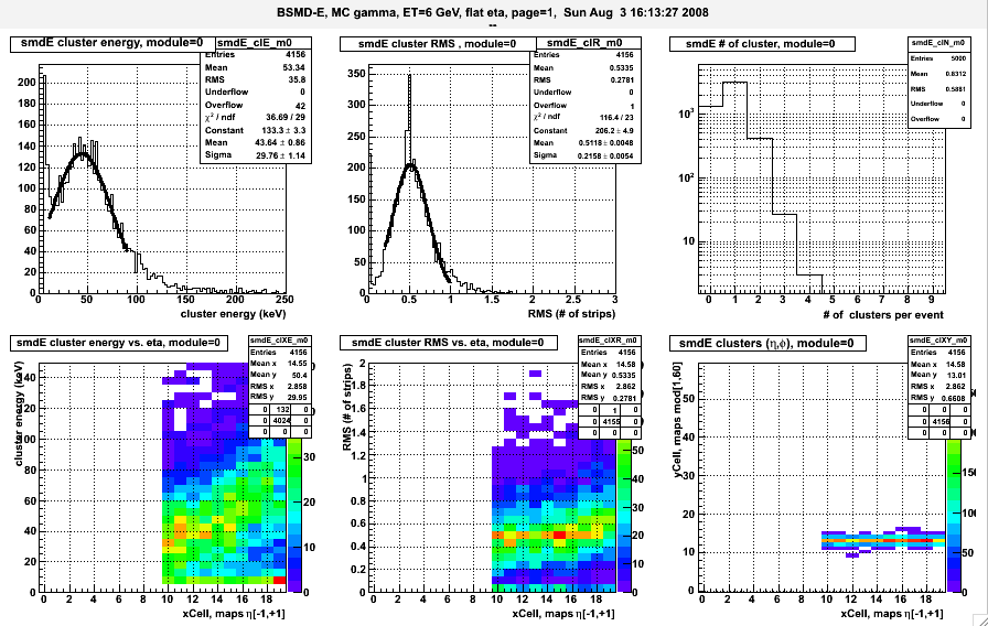
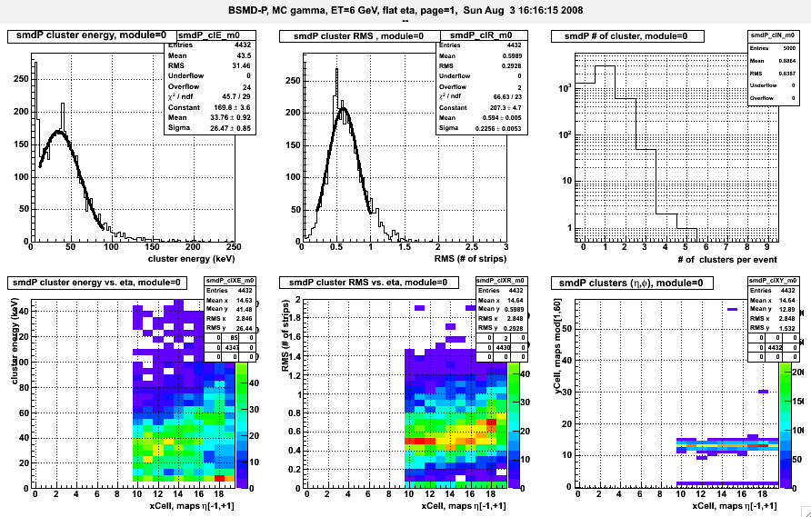
4) demonstration of absolute calib algo on single particle M-C
Goal: determine absolute calibration of BSMDE,P planes
Method: identify isolated EM shower and match BSMD cluster energy to tower energy
INPUT events: single particle per event, fixed ET=6 GeV, flat eta [-0.1,1.1], flat |phi| <5 deg, 5k eve per sample, Geant geometry y2006
Cluster finder algo (seed is sliding fixed window), tuned on pi0 events
- work with 150 Eta-strips per module or 900 Phi-strips at fixed eta
- all strips are marked as 'unused'
- use only module 13, covering ~1/3 of probed phase space
- sum geant dE in fixed window of 3 unused strips, snap at location which maximizes the energy
- if sum below 5 keV STOP searching for clusters in this module
- add energy from one strip on each side, mark all 1+3+1 strips as 'used'
- compute energy weighted cluster position and RMS
- goto 1
This cluster finder process full Barrel West, more details about clustering is in one cluster topology , definition of 'barrel cell'
Isolated EM shower has been selected as follows, tuned on gamma events,
- select isolated eta-cluster in every segment of 15 eta strips.
- require cluster center is at least 3 strips away from edges of this segment (defined by eta values of 0.0, 0.1, 0.2,....0.9, 1.0)
- require there is only one phi-cluster in the same 0.1x0.1 eta.phi cell
- require phi-cluster center is at least 3 strips from the edges
- find tower matching to the cross of eta & phi cluster
- require this tower has ADC>100
Example of EM cluster passing all those criteria is below:
smdE: ene/keV= 40.6   inTw 451.or.471
 cell(15,12),   jStr=7 in xCell=15
...
id=1731  ene/keV=4.9  *
id=1732  ene/keV=34.3  X *
id=1733  ene/keV=1.5  *
...
---- end of SMDE dump


smdP: ene/keV= 28.5  inTw 471.or.472
  cell(15,12),   jStr=7 in xCell=15
...
id=1746  ene/keV=2.7  *
id=1756  ene/keV=22.0  X *
id=1766  ene/keV=3.7  *
...
---- end of SMDE dump

muDst BTOW
  id=451, m=12 rawADC=12.0
* id=471, m=12 rawADC=643.0
  id=472, m=12 rawADC=90.0
  id=473, m=12 rawADC=10.0
Results for gamma events
will be show with more details. The following PDF files contain full set of plots for all other particles.
particle | # of eve | plots |
| gamma | 25K | |
| e- | 50K | |
| pi0 | 50K | |
| eta | 50K | |
| pi- | 50K |
Fig 1, Any Eta-cluster, single gamma, 25K events
TOP: a) Cluster (Geant) energy; b) Cluster RMS, c) # of cluster per event,
BOTTOM: X-axis is eta location, 20 bins span eta [-1,+1]. d) cluster ene vs. eta, e) cluster RMS vs. eta, f) cluster yield vs. eta & phi.

Fig 2, Any Phi-cluster, single gamma, 25K events
see Fig 1 for details

Fig 3, Isolated EM shower, single gamma, 90K events
TOP: a) cluster loss on subsequent cuts, b) # of accepted EM cluster vs. eta location, c) ADC distribution of hit tower (some wired gains are in default M-C), tower ADC is in ET
BOTTOM: X-axis is eta location, 20 bins span eta [-1,+1]. d) Eta-cluster , e) phi-cluster energy, f) hit tower ADC .

Fig 4, Calibration plots, single gamma, 90K events.
TOP: BSMD Eta vs. Phi as function of pseudorapidity. BOTTOM: BSMD vs. BTOW as function of pseudorapidity.3 eta location of 0.1, 0.5, 0.9 of reco EM cluster are shown in 3 panels (2x2)
1D plots are ratios of the respective 2D plots.
The mean values of 1D fits are relative gains of BSMDP/BSMDP and BSMD/BTOW , determine for 10 slice in pseudorapidity. Game is over :).

Fig 5, Same as above, eta=0.1, single pi0, 50K events.

Fig 6, Same as above, eta=0.1, single pi minus, 50K events.

Below are PDF plots for all particles:
Correction - label on the X-axis for 1D plots is not correct. I did not apply log10() - a regular ratio is shown, sorry.
5) Evaluation of BSMD dynamic range needed for the W program at STAR, ver 1.0
M-C study of BSMD response to high energy electrons

Attachment 1:
Fig 1 & 2 reminds actual (pp data based) calibration for 2 eta location of 0.1 and 0.8, presented earlier.
Table 1 shows M-C simulation of average cluster energy (deposit in BSMD plane), its spread, and width as function of electron ET, separately for eta- & phi-planes of BSMD.
As expected, BSMD sampling fraction (SF, red column) is not constant but drops with energy of electron.
The BSMD SF(ET) deviates from constant by less then 20% - it is a small effect.
Fig 3,4,5 show expected BSMD response to M-C electrons with ET of 6,20, and 40 GeV. Only for the lowest energy the majority of EM showers fit in to the dynamic range of BSMD, which ends for energy deposit of about 60 keV per plane.
I was trying to be generous and draw the red line at DE~90 keV .
The rms of BSMD cluster is about 0.5 strips, so majority of energy is measured by just 2 strips (amplifiers). Such narrow cluster lowers saturation threshold.
Fig 6, shows BSMD cluster energy for PYTHIA W-events.
Fig 7 shows similar response to PYTHIA QCD events.
Compare area marked with red oval - there is strong correlation between BSMD energy and electron energy and would be not wise to forgo it in the e/h algo.
Conclusion:
The attached slides show 2008 HV setting of BSMD would lead to full saturation of BSMD response for electrons from W decay with ET as low as 20 GeV , i.e. would reduce BSDM dynamic range to 1 bit.0
For the reference:
* absolute BSMD calibration based on 2008 pp data.
http://drupal.star.bnl.gov/STAR/subsys/bemc/calibrations/bsmd/2008-bsmd-calibration/19-isolated-gamma-algo-description-set-2-0
* current BSMD HV are set very high , leading to saturation of BSMD at gamma energy of 7-10 GeV, depending on eta and plane. (Lets ignore difference between E & ET for this discussion, for now).
http://drupal.star.bnl.gov/STAR/subsys/bemc/calibrations/bsmd/2008-bsmd-calibration/20-bsmd-saturation
* STAR priorities for 2009 pp run presented at Apex: http://www.c-ad.bnl.gov/APEX/APEXWorkshop2008/talks/Dunlop_Star_Apex_2008.pdf
* Attachment 2,3 show BSMD-E, -P response for electrons with ET: 4,6,8,10,20,30,40,50 GeV and to Pythia W, QCD events (in this order)
BSMD 2005 energy scale uncertainty
STAR/blog/ogrebeny/2009/jun/08/bsmd-energy-scale-uncertainty
Definition of absolute BSMD calibration
NOT FINISHED
Definitions of quantities used for empirical calibration of BSMD.
Revised January, 26, 2009
A) Model of the physics process (defines quantities: E, eta, smdE, smdEp, smdEe, C0, C1)
- gamma particle with fixed energy E enters projectively EMC at fixed pseudo-rapidity eta. Eta is defined in detector ref. frame.
- EM showers develops and BSMD (consisting of 2 planes) captures smdEtot of shower energy. Single plane captures smdE=0.5*smdEtot. The SMD cluster energy from single plane is denoted as smdE.
- SMD consist of 2 planes : eta-plane closer to IP and the outer phi-plane. Each plane captures non-equal fraction ofenergy deposited in BSMD: smdEp, smdEe, respectively.
 The following relation holds:
smdEp(E,eta) =smdE(E) * [1-C1(eta)]
smdEe(E,eta) =smdE(E) * [1+C1(eta)]
where theta-dependent coefficient C1 accounts for all physical processes differentiating fraction of captured shower energy by eta vs. phi-planes along Z-direction.
allows reconstruction of full BSMD energy deposit independent on gamma angle theta if cluster energy in both plane is measured - BSMD Cluster energy is measured in each plane by few consecutive strips which:
- response is linear and
- strip-to-strip local hardware gain variation is negligible (the "long-wave" is accounted for in C1(theta))
Note, there are 4 low gain strip (id=50,100) in the eta-plane , seen in fig 2 of 08) SMD-E gain equalization , ver 1.1, which require ADC to be rescaled appropriately.

- The overall conversion constant C0=6.5e-8 (GeV/ADC chan) allows reconstruction of BSMD cluster energy in given plane based on the sum of ADCs from all strips participating in the cluster
smdEp(E,eta)=C0* sum{ ADC_i - ped_i}, over cluster of few strips , similar formula for smdEp(E,eta)=....
The value of C0 was determined based on 19) Absolute BSMD Calibration, table ver2.0, Isolated Gamma Algo description, table 2. Gammas with ET=6 GeV were thrown at EMC and resulting SMD cluster ADC sum was matched to the average value seen for 2008 pp data.
To summarize
The reconstructed cluster energy in each plane with use of C0 & C1 should have eta dependence
smdE(E) =C0* sum{ ADC_i - ped_i}/[1-C1(eta)] for phi-plane cluster
smdE(E) =C0* sum{ ADC_j - ped_j}/[1+C1(eta)] for eta-plane clusterThose 2 quantities are well suited to place cuts.
B) Determination of C1(eta) was based on 19) Absolute BSMD Calibration, table ver2.0, Isolated Gamma Algo description, from crates 1,2,and 4.
Data analysis was done for 10 pseudo-rapidity ranges [0,0.1], [0.1,0.2] ,..., as shown in table 2, row labeled 'DATA'.
For practical application analytical approximation is provided
C1(eta)= C1_0 + C1_1*|eta| + C1_2*eta*eta
symmetric versus positive/negative pseudo-rapidity.
The numerical values of expansion coefficients are: C1_0=0.014, C1_1=0.015, C1_2=0.333
C) Modeling of BSMD response in STAR M-C
- find geantDE geant energy deposit for given BSMD strip
- undo simulated by GEANT +/-7% difference between eta/phi planes (see 19) Absolute BSMD Calibration, table ver2.0, Isolated Gamma Algo description, row 'M-C')
geantDEp=geantDE*0.93
geantDEe=geantDE*1.07 - compute ADC for every i-th strip & plane
ADCp_i= geantDEp/[1-C1(eta)]/C0
ADCe_i= geantDEe/[1+C1(eta)]/C0- If NO saturation is assumed that is all - use ADC-values in reconstruction.
- To simulate full ADC saturation at 1024 assume pedestal is at ADC=100 and saturate values of ADCp_i, ADCe_i at 924. Then proceed to reconstruction.
Mapping, strip to tower distance
For every strip we find the closest tower and determine the distance between tower center and strip center.
Both plots show strip ID on the X-axis, and tower ID on the Y-axis. Error in Y is distance between centers in CM.
It is not true 15 eta strips covers every 2 towers! It is only approximate since strip pitch is constant bimodal and tower width changes continuously.
There is still small problem, namely strip Z is calculated at R_smd and tower Z is calculated at the entrance of the tower
leading to clear paralax error - we are working on this.
Fig 1.
Top plots is for SMDE for module 1. Note E-strip always spans 2 towers and we used tower IDs in one module.
Bottom plots shows phi strips for module 1.

Fig 2.
Top plots is for SMDE for modules 1-4.
Bottom plots shows phi strips for modules 1-4.


Run 10 BSMD Calibrations
Parent page for BSMD Run 10 Calibration
BSMD Status Table in run10 AuAu200GeV runs
==========
We started this task by looking at BSMD in Run 10 with some MuDst files, and found the pedestals probably need to be QA-ed as well.
http://www.star.bnl.gov/HyperNews-star/get/emc2/3500.html
and
http://www.star.bnl.gov/HyperNews-star/get/emc2/3515.html
==========
Then we started to look for Non-zero-suppressed BSMD data, and found that we have to run through the daq files to produce the NZS data files to produce the NZS data. The daq files are stored on HPSS, and we have to transfer them onto RCF. The transferred daq files were then made into root files with Willim's BSMD online monitering codes.
http://www.star.bnl.gov/HyperNews-star/get/emc2/3533.html
==========
We decided to use same critiria and status codes as Willim used for run09 pp500GeV.
http://drupal.star.bnl.gov/STAR/blog-entry/wleight/2009/may/13/bsmd-status-cuts-and-parameters
==========
We discovered that a modification is needed to the critiria of code bit 3 (the ratio of the integral over a window to the integral over all, i.e. the pedestal integral ratio) We found about half of the BSMD strips fail the criteria of this ratio > 0.95, but nearly most of them satisfy ratio > 0.90, so the critiria is loosed to 0.90. We think this is a reasonable difference between run09 pp and run10 AuAu collisions.
http://www.star.bnl.gov/HyperNews-star/get/emc2/3546/1/1.html
==========
The daq files are huge in size, on the order of TB for one day. In order to not disturb the run10 data production, we had to only copy 1/10~1/20 of the daq files.
http://www.star.bnl.gov/HyperNews-star/get/emc2/3589/2.html
==========
After a long period of transffering and root files making, almost all the days between Jan/02/2010 and Mar/17/2010 are done.
http://www.star.bnl.gov/HyperNews-star/get/emc2/3601.html
We found that another criteria has to be modified, because we use NZS data for the QA of the tail of ADC spectrum. The definition of the tail ranges and the limits are adjusted. Three ranges of the tail part of ADC are defined,
Range 1:peak+6*rms to peak+6*rms+50 channels
Range 2:6*rms+50 channels to 6*rms+150 channels
Range 3:6*rms+150 channels to 6*rms+350 channels
The entries (hits) in these three ranges are counted, and the ratios to all the entries in the whole spectrum are calculated. The limits for good ratios are selected based on the ratios distribution trough out all the days. They are
@font-face {
font-family: "Cambria";
}p.MsoNormal, li.MsoNormal, div.MsoNormal { margin: 0in 0in 0.0001pt; font-size: 12pt; font-family: "Times New Roman"; }div.Section1 { page: Section1; }
Range 1: 3.35~80 x0.001
Range 2: 0.95~40 x0.001
Range 3: 0.25 ~ 20 x0.001
See the attached newlimits.docx for more details and plots.
Also, bit 0 of the status code is supposed to indicate whether a channel is bad or not. Not every problem is fatal, i.e cause the channel to be regarded as bad.
Originally, only if all the 3 ratios are beyond the limits, a fetal condition is met; we addjusted this to be if more than one, i.e. >=2, out of the 3 ratios are beyond the limits, a fetal condition is met. One can also treat any channel with a code not equal to 1 as bad, regardless what the bit 0 is.
==========
A final report with sample codes in one day was presented to and approved by EMC2 group.
http://www.star.bnl.gov/HyperNews-star/get/emc2/3637/1.html
==========
Note: The map file used in bsmd montoring in run10 was with some inconsistence with the acctual hardware. An after-burn map correction was done by the EMC software coordinator, Justin.
Note: Up to now, no corrections are made to pedestals. The bad strips caused by bad pedestals are rouphly 1/3~1/4 of all the bad strips.
Wenqin Xu
16Feb2011
Run 9 BSMD Calibration
Parent page for BSMD Run 9 Calibration
01 Status of BSMDE,P at the end of pp 500 GeV run, April of 2009
Summary of BSMD performance on April 6. Input : 200K events tagged by L2W clust ET>13 GeV, days 85-94, ~all events, only ZS data are shown.


Attached PDFs shows zoom in spectra for individual modules. 1st page is summary, next I show 3 modules per row, 5 rows per page. Even pages shows zoom-in for low ADC<100, odd pages shows full ADC scale. Common maxZ=1000 is used for all plots , except page 1.
02 offline QA of BSMD pp 500, ver1 (Willie+Jan)
BSMD QA algorithm and results for pp 500, tune optimized for high energy energy response
- QA method, details are given in Willie's blog
Fig 1. Typical good/bad strips from the E-plane and with wide pedestals.

- Input: all available events from fills 10399, 10402, 10403, 10404, 10407, 10412, 10415 added together
- evaluate shape of pedestal residua for NZS data captured on-line by Willie's daq reader (Blue filled histo)
- evaluate yield in high energy range (ADC ~300,500,800) using ZS data from L2W triggered events (Magenta line-only)
- ignored: satellite spikes around pedestal at ADC ~32, those come from correlated noise and (most likely) such events will be discarded.
- Example of such spectra for few strips is shown in fig 1.
- Encoding of BSMD status bits extends existing convention to use LSB=1 for good strips and LSB=0 for bad strips. We used bits 1,2,3 to tag pedestal problems and bits 5,6,7 to tag yield problems.
- More plots with individual strips is in attachment A,B,C,D.
- Bad strip is defined as having : bad pedestal or god pedestal but no yield above it.
Fig 2. Distribution of bad strips from both planes, details about each plane separately is in attachment E.

- The remaining issues:
- of tagging 'spiked' events (or modules?) needs to be investigated.
- study time dependence
- For the reference this directory contains PDF files with plots from all 120 BSMD modules.
Fig 3. # of bad strips per module.

03 correlated, small ADC spikes in BSMD (Jan)
Study of small ADC spikes in BSMD
Input:
The following plots support those observation:
- spikes are symmetric on both sides of pedestals peak, separated by 2^N ADC counts, narrower than pedestal peak, (Fig1)
- spikes are correlated in even ID (or odd) strips the same plane, correlation is local, Fig 2
- spikes are correlated between P-plane & E-plane strips, Fig 3
- energy deposit in BSMD increases probability of spikes, see peak/valley for blue vs. magenta in fig 1b.
- bands are visible at larger ADC, as shown by Oleg, not sure what data and how many events, fig 4
- perhaps fig 1c shows yet another pathology, because it does not obey odd/even rule in fig 1a & 1b.
Fig 1a. Example of spikes delADC=16, in the vicinity of strip 1525-P, all strips from module 11 are shown in attachment A.

Fig 1b. Example of spikes delADC=32, in the vicinity of strip 1977-P, all strips from module 14 are shown in attachment B, module 22 looks similar.

Fig 1c. Example of spikes delADC=128, in the vicinity of strip 4562-P, all strips from module 31 are shown in attachment C, modules 51,52,57 look similar

Fig 2. Phi-Phi plane correlation of P-strip 1979 with (odd) P-strips: 1977..1994. Attachment D contains correlation of P-strips [1977-80] with 24 strips in proximity.

Fig 3. Phi-Eta plane correlation of P-strip 1979 with (odd) E-strips: 1977..1994. Attachment E contains correlation of P-strips [1977-80] with 24 strips in proximity.

Fig 4.Oleg observed this stripes in raw BSMD ADC spectrum, not sure what data.

2009 BSMD Relative Gains Information
The pdf posted here has a good overview of the computation of the slope for each strip, discussing the method and the various ways in which strips were marked as bad. This page discusses the computation of the actual relative gains and statuses that went into the database.
The code used to compute the relative gains is archived at /star/institutions/mit/wleight/archive/bsmdRelGains2009/.
DELETE - Run 9 BSMD Status Update 3 (4/24)
After looking more closely at the crate 1 channels I was forced to make serious revisions to status bit 2 from the previous update. The new status bit 2 test is as follows:
First, I scan through the strip ADC distribution looking for peaks. A peak is defined as a channel that is greater than or equal to the four or two channels to either side (if the sigma of the fit to the strip ADC distribution is greater than or less than six, respectively), has a content that is greater than 5% of the maximum of the strip ADC distribution, and has a depth greater than 5% of the maximum of the strip ADC distribution. The depth is calculated by first calculating the difference between the peak content and the channel content for each of the four or two channels on either side of the peak. The maximum of these differences is obtained for the left and right sides separately, and the depth is then equal to the lesser of these two maxima.
If the strip has more than one peak and the maximum of the depths is greater than 20% of the maximum of the strip ADC distribution, then the strip is given bad status 2. If the strip has only one peak (which is then necessarily the maximum of the entire distribution) but the distance between that peak and the peak obtained from the gaussian fit is greater than 75% of the sigma from the gaussian fit, the strip is given bad status 2 as well. Attached is a pdf that has only the pedestal plots for all channels from crate 1.
Edit: I forgot that the BSMD crates don't increase with module number: what is labeled as crate 1 is actually crate 2, as that is the crate that has the first 15 modules, and the attachment labeled as crate 2 is the 2nd 15 modules and so actually crate 1.
2nd edit: This is now out of date, please see the new update.
DELETE - Run 9 BSMD Status Update 4 (4/27)
After further investigations -- specifically looking at strips that had a significant secondary peak, entirely separated from the main peak, with a max of ~40, which were not being caught by my cuts -- I have again revised my criteria for status bit 2. Again, I begin by looking for peaks. If a peak candidate is less than three sigma from the peak of the strip ADC distribution (strip and peak both taken from the gaussian fit), the same cuts are imposed: the candidate must be greater than the four (if sigma>6) or two (if sigma<6) channels on on either side of it, it's content must be greater than 5% of the maximum of the strip ADC distribution, and the depth must be at least 5% of the maximum of the strip ADC distribution. If the strip has two such peaks with the maximum of the depths greater than 20% of the maximum of the strip ADC distribution, or has only one peak but that peak is at least one sigma away from gaussian fit peak, it is given bad status 2. Note the only change here is that the previously a strip with only one peak could be marked bad if it was 75% of sigma away from the gaussian fit peak.
Most of the changes have to do with candidates that are at least three sigma from the gaussian fit peak. In this case the cuts are relaxed: the bin content need only be .5% of the max, not 5%, though it still must be at least 10, and the peak depth is required to only be at least 5% of the peak itself, not of the max. A more than three-sigma peak has the same requirements for the number of channels it must be greater than: however, none of those channels can have value 0. Any strip with a candidate that passes these criteria is automatically given bad status 2.
Pdfs for crates 1 and 2 are attached (but note that the crate 1 and crate 2 pdfs contain the first and second 15 modules, respectively, and therefore crate 1 should actually be labeled crate 2 and crate 2 is really crate 4).
DELETE - Run 9 BSMD Status Update 5 (4/30)
Edited on 5/1 to reflecte new status bit assigments for bits 3 and 4.
The current BSMD status bits are as follows:
Bit 2: Bad pedestal peak/multiple pedestal peaks. This is described in more detail here. Examples can be found in crate2_ped.pdf pp 207 and 314 and crate4_ped.pdf p 133.
Bit 3: Pedestal peak has bad sigma, sigma<1 or sigma >15
Bit 4: Chi squared value from gaussian fit is greater than 1000 (i.e., pedestal has a funny shape)
Bit 5: Strip is exactly identical to the previous strip
Bit 6: The ratio of the integral of channels 300-500 to the total integral does not fall between .0001 and .02
Bit 7: The ratio of the integral of channels 500-800 to the total integral does not fall between .00004 and .02
Bit 8: The ratio of the integral of channels greater than 800 to the total integral does not fall between .00005 and .02
Note that this means that dead channels have status 111xxxx0->448 (or greater).
The attached pdfs crate2 and crate4.pdf have the pedestal distributions, taken from NZS data, and the overall distributions, taken from ZS L2W data, overlayed; crate2_ped and crate4_ped.pdf have only the pedestal distributions. The NZS data used was taken from my monitoring for fills 10415-10489. The L2W data came from fills 10383-10507. Additionally, at the beginning of each module is a summary page that has plotted the distributions for the ratios used to determine bad status bits 6, 7, and 8, and the overal distribution of status vs. strip for eta and phi.
Finally, there are a couple of possible new problems. Page 18 in crate4_ped.pdf has several examples of pedestal distributions that have shoulders. Page 20 has a few examples of pedestal distributions with a small, skinny peak perched on top of a large, broad distribution. At the moment I have no bad status bit for either of these, and any peak with either of these features would almost certainly not be marked bad (even though I did manage to catch one of the ones on page 20).
Edit: Scott suggested during the phone meeting today that perhaps the problem of a small peak on a broad distribution was due to time variation of the pedestal width, and in the plot below you can see that he was correct: the strip initially has an extremely wide pedestal which then shrinks down suddenly. Futhermore, looking at one of the strips that had a sort of shoulder to it, you can see that this is just a less-pronounced version of the double peak problem seen before: the pedestal goes up by 10 for a much shorter time frame, thus producing a shoulder rather than a second peak. This suggests that, as Scott said, these channels should still be usable, and that once we begin breaking status down by time these funny shapes should be less of a problem.


DELETE - Run 9 BSMD Status Update 6 (5/4)
As Matt says that the maximum status is 255, I have dropped the old status bit 5 as (it was unused). Also, I have loosened the dead strip cuts based on looking at module 55 (see pages 203 or 205 in the attached crate1.pdf, for instance). The status bits are now as follows:
Bit 2: Bad pedestal peak/multiple pedestal peaks.
Bit 3: Pedestal peak has bad sigma, sigma<1 or sigma >15
Bit 4: Chi squared value from gaussian fit is greater than 1000 (this applies only for strips that do not have bad status 2 already)
Bit 5: The ratio of the integral of channels 300-500 to the total integral does not fall between .0005 and .02
Bit 6: The ratio of the integral of channels 500-800 to the total integral does not fall between .0002 and .02
Bit 7: The ratio of the integral of channels greater than 800 to the total integral does not fall between .0002 and .02
Below is a plot of status vs. eta and phi for BSMDE and BSMDP strips. Note that strips with all three of bits 5, 6, 7 bad (generally, dead strips) are given the value 8 in this plot to distinguish them from strips that may have just one of those bits bad. As some strips may have more than one bad status bit, for clarity I ranked the potential bad statuses in the order 2, 8, 7, 6, 5, 4, 3 (i.e., approximately in order of importance) and plotted for each strip only the highest-ranked status.

Additionally, I found a problem I had not seen before. On page 207 of the attached crate1.pdf you can see that in the L2W data some strips have a large peak out in the tail of the ADC distribution. However, as all these strips are caught by my code it's not a serious problem.
Final Run 9 200 GeV BSMD Status
In essence, the 200 GeV status tables were calculated the same way as the 500 GeV tables were. Please see here for details.
Final Run 9 500 GeV BSMD Status - Willie Leight
BSMD Pedestals and Status for Run 9 pp 500 Data (June 2009, uploaded to offline DB)
The BSMD status analysis for the 500 GeV data proceeds as follows:
- Each strip is assigned a status for the whole run from an analysis of fills 10399, 10402, 10403, 10404, 10407, 10412, and 10415. Pedestals are analyzed using NZS data taken by the BSMD online monitoring, which reads NZS data from evp and subtracts off pedestals which are updated each time a new BSMD pedestal run is taken. Because NZS data is essentially minbias, high energy tails are analyzed using L2W-triggered data. Status bits are described in detail here.
- Once each strip has an assigned status, those strips that are not marked as bad move on to the second step. Here the strips are examined fill-by-fill: for each fill the strip pedestal is QAed by re-applying the pedestal cuts (but not the tail cuts due to lack of statistics), and a new status for that fill is determined.
- Next, a pedestal correction is calculated. The pedestal correction is just the MPV of the pedestal residua if the MPV is greater than the RMS of the pedestal residua.
- Finally, we upload a number of tables to the database: for each BSMD plane there is one that contains a universal status for every strip, one for each fill containing a status for every strip, and one for each fill containing the RMS and pedestal correction for every strip.
Attached is a pdf that presents the results of this study, including examples.
All code and root files are archived at /star/institutions/mit/wleight/archive/2009-pp500-bsmdStatus/.
Table 1: Pedestal correction, RMS, and status vs. fill for each module (Crates 1-4 are the West Barrel)
Table 2: BSMD spectra for 150 eta and 150 phi strips used for status determination for each module (for fills listed above). Bad strips are identified with the status (in hex): strips with red status are marked bad, strips with green failed a cut but are not necessarily bad. Note that these spectra are shifted up by 100 on the X-axis so that the pedestal is centered around 100 rather than 0.
Table 3: Fills used in this study.
# Fill Date Begin run End run LT/pb
1 F10383 2009-03-18 R10076134 R10076161 0.00
2 F10398 2009-03-20 R10078076 R10079017 0.08
3 F10399 2009-03-20 R10079027 R10079086 0.22
4 F10402 2009-03-21 R10079129 R10079139 0.04
5 F10403 2009-03-21 R10080019 R10080022 0.01
6 F10404 2009-03-22 R10080039 R10080081 0.09
7 F10407 2009-03-22 R10081007 R10081056 0.05
8 F10412 2009-03-23 R10081096 R10082095 0.23
9 F10415 2009-03-24 R10083013 R10083058 0.24
10 F10426 2009-03-25 R10084005 R10084024 0.11
11 F10434 2009-03-26 R10085016 R10085039 0.18
12 F10439 2009-03-27 R10085096 R10086046 0.26
13 F10448 2009-03-28 R10087001 R10087041 0.29
14 F10449 2009-03-28 R10087051 R10087097 0.32
15 F10450 2009-03-29 R10087110 R10088036 0.29*
16 F10454 2009-03-29 R10088058 R10088085 0.15*
17 F10455 2009-03-30 R10088096 R10089023 0.29*
18 F10463 2009-03-31 R10089079 R10090027 0.20*
19 F10464 2009-03-31 R10090037 R10090047 0.08*
20 F10465 2009-03-31 R10090071 R10090112 0.13*
21 F10471 2009-04-02 R10091089 R10092050 0.30
22 F10476 2009-04-03 R10092084 R10093036 0.28
23 F10478 2009-04-03 R10093057 R10093085 0.08
24 F10482 2009-04-04 R10093110 R10094024 0.55
25 F10486 2009-04-05 R10094063 R10094099 0.52
26 F10490 2009-04-05 R10095019 R10095057 0.40
27 F10494 2009-04-06 R10095120 R10096027 0.61
28 F10505 2009-04-07 R10096139 R10097045 0.39
29 F10507 2009-04-08 R10097086 R10097153 0.29
30 F10508 2009-04-08 R10098029 R10098046 0.17
31 F10517 2009-04-09 R10099020 R10099078 0.32**
32 F10525 2009-04-10 R10099185 R10100032 0.68
33 F10526 2009-04-10 R10100049 R10100098 0.37
34 F10527 2009-04-11 R10100164 R10101020 0.82
35 F10528 2009-04-11 R10101028 R10101040 0.31
36 F10531 2009-04-12 R10101059 R10102003 0.86
37 F10532 2009-04-12 R10102031 R10102070 0.76
38 F10535 2009-04-13 R10102094 R10103018 0.86
39 F10536 2009-04-13 R10103027 R10103046 0.43
* Crate 2 was off for this fill
** This fill had no BSMD data
Final Run 9 BSMD Absolute Calibration
The Run 9 BSMD absolute calibration was made using few-GeV TPC-identified electrons from pp500 running, and has two pieces. The first is a new CALIBRATION table in the database which will be used in the EMC slow simulator to improve the agreement of of MC ADC with data. This table starts by combining the previously-determined strip-by-strip relative gains with the existing values in the table. This is then multiplied by the ratio of the slope of a linear fit to the mean cluster ADC distribution from few-GeV isolated data electrons to the same slope in simulated electrons, where the slope is calculated in four different eta bins. The second piece is a new GAIN table in the database which allows ADC values to be converted to energy deposited in the BSMD. This table was determined by combining the strip-by-strip relative gains with a similar ratio as above, but using mean cluster energy deposited in the BSMD instead of reconstructed ADC values (the electron samples used for data and MC were the same) and it is calculated in ten eta bins instead of four. Both tables are currently in the database with flavor "Wbose2": it is hoped that eventually the CALIBRATION table will migrate to flavor "ofl", but the GAIN table will have to remain "Wbose2" because it is currently used (with values all equal to 1) in some codes to determine the change in the BSMD calibration over time. While producing two tables which are in some ways overlapping and one of which can never be flavor "ofl" is not an ideal solution, it allows us to avoid making any modifications to currently existing code (in particular the StEmcSimulator) and allows people who prefer to think of reconstructed energy from BSMD ADCs as being the full particle energy instead of the energy deposited in the BSMD to continue as they were with no change. For more details, please see:
2. Final cut list and data-MC comparison
Additionally, a link to the 2009 BSMD Calibration note will be added here once it is completed.
See also a brief presentation on why we chose not to include the BSMD gas pressure in our analysis.
Run 9 BSMD Status Update 1 (4/19)
I use two datasets to QA BSMD channels: zero-suppressed data from L2W events (fills 10383-10507) and non-zero-suppressed data from online monitoring (fills 10436-10507) (note that at the moment I am not examining the time dependence of BSMD status). NZS data is used to QA the pedestal peak of a channel, while high-energy ZS data is used to QA the tail.
Next, the ZS data are compared to the ZS data from the previous channel to check for copycat channels. Then three quantities are calculated: the ratios of the integrals from 300-500, 500-800, and 800-the end of the spectrum to the total integral of the channel. Each of these quantities must then fall within the following cuts: .0001-.02, .00004-.02, and .00005-.02 respectively. Here is a sample distribution:

Also, the spectra for the strips in module 3, with status, are attached. I have not had a chance to look closely at any other modules yet.
details about known hardware problems
Attached file 'SMD_07.xls' contain my notes from run 7, the only things that might be useful for
you is in the red color, permanently disconnected anode wires and affected
strips (again this is not SoftIds). I think that I cut out one more wire
before Run8 started, but for that I need to check logbook.
Oleg
-----------------------
BSMD Wire Support Effects on GAIN
Here is a note from Oleg Tsai (and attached file "wiresup.pdf" below) concerning source
measurements of the BSMD gain behavior near the nylon wire supports:
On Fri, 18 Jul 2008, tsai@physics.ucla.edu wrote:
> Attached plot will help you to understand what you see close to
> strips 58 and 105. There are two nylon wire supports in the chamber
> at distances 34.882" and 69.213" from the (eta=0 end of the chamber,
> not from the real eta 0). Gain drops near these supports. You can
> see this in your plots also. The attached plot shows counting rate vs
> strip id for a typical chamber. Don't pay attention to channels
> near 0 and 150 - these effects are due to particular way co60 source
> was collimated (counting profile was close to 0.1/0.2/0.4/0.2/0.1)
> 0.4 in central strip. From that I estimated that eta strips
> 56-60 and 104-107 should have calib. coefficients
> (.95,.813,.875,.971,.984) (.99,.89,.84,.970.), I don't remember
> if I was using counting rate vs HV to derive these numbers...
> (this is my third and final attempt :-))
>
details of SMD simulator, simu shower zoom-in
Fig 1. Geant simu of EM shower of one electron with ET=10 GeV at eta=0.
Note,
- one phi-strip is parallel to cavities, extends over 1/10 of the cavity length, and integrates over 2 consecutive cavities.
- one eta-strip is perpendicular to cavities, extends over 1/150 of the cavity length, and integrates over all 30 cavities in the module.

Hi Jan,
the only documentation I know of is the code itself --
hopefully you'll consider it human-readable. Look at
StEmcSimpleSimulator::makeRawHit() in StEmcSimulatorMaker. We use the
kSimpleMode case. The GEANT energy deposition is multiplied by a
sampling fraction that's a second-order polynomial in pseudorapidity,
and then we take pedestals, calibration jitter, etc. into account.
The exact parameters of the sampling fraction are defined in the
constructor for StEmcSimpleSimulator. I don't remember how they were
determined.
also meant to add that the width broadening is OFF by
default. To turn it on one needs to do
emcSim->setMaxCrossTalkPercentage(kBarrelEtaStripId, aNumber);
The "width broadening" only occurs
for eta strips and was implemented by Mike Betancourt in
StEmcSimulatorMaker::makeCrossTalk(). He wrote a blog post about it:
http://drupal.star.bnl.gov/STAR/blog-entry/betan/2007/nov/19/cross-talk-bsmd
Adam
Maybe I should note that the cross talk I implemented was to account
for the capacitive cross talk between the cables carrying the eta
strip signals to the readout, and not for any effects related to the
energy deposition.
-Mike
Hi Jan,
Well, Oleg should probably make the definitive reply, but I think it is like this:
The amplification happens only at the wire, it is independent of the positions of the primary ionization. Of course, there is a little effect from a small amount of recombination or capture of the charge on impurities, and there must be a (hopefully small) effect from the dependence of the mean pulse shape on the position of the ionization and the dependence of the effective gain of the electronics on the mean pulse shape. But these things can't amount to much, I would think. (Of course, I don't want to discourage you from looking in the data to confirm it!)
Gerard
These are all quite true, small effects which will be difficult
to see. The bigger effect is reading out one time bucket.
I have made some estimates before test run 98 (?) or so, see this PS
if you look at numbers still very small effect which is unpractical
to measure.
Oleg
Hi, Yes indeed, I don't know why I neglected to think of the simple effect of drift time, but it is certainly going to be a much bigger effect (~10% if I read your fig.3 correctly?) than the other two. (Perhaps still too small to see in the data, I don't know...). Anyway, given the data volume and already limited readout speed of the BSMD I am pretty sure there is no prospect to ever read more than the one fixed time sample from BSMD; this is probably something to live with. [But it is not impossible to have 2 or 3 point readout, and if we want to seriously consider it it should be brought up ~now, well that is in case we are given the green light to work on BSMD readout "mini-upgrade". If not, well it will just wait until then. But keep in mind, more points readout would offer slightly better gain accuracy but will complicate offline and calibrations too, probably you really don't want it anyway!]
Gerard
p.s. Jan I don't know if it adds anything to the wider discussion on BSMD gain/cal but if you feel so you may surely post to hn.
p.p.s. Oleg, an important question - in your note you don't specify exactly how you obtain the drift time... I mean, yes you show a drift velocity curve, but really of course you must mean there was a calculation such as with garfield to get a drift time out of this... _So_, was that calculation done with the magnetic field on? [The wires are parallel to the magnetic field, right? So it will make possibly a very big difference in drift times.] Jan, do you/others realize the BSMD gain will probably have some systematic dependence on the magnetic field, including the sign thereof? So if you care about gain calibration it should be separated out according to the state of STAR magnet, fortunately there are only a few running states, right?
Gerard
one cluster topology , definition of 'barrel cell'
One dimensional BSMD cluster finder is insensitive to single dead strips and module boundaries for the phi strip.
However certain class of Phi-strip clusters (marked as red) are artificial split and reco as 2 phi-clusters.
One could use the Eta-strip cluster to recover from such phi-plane split if occupancy is low and relative scale of eta & phi cluster energy known.
Plots below also introduce a concept of 'barrel cell' which has approximate size of 0.1 in eta & phi physical units and is aligned with barrel modules. 'barrel cell' is the smallest common unit in eta-phi space for SMD and BTOW tower topologies.
'Barrel cell' has 2 coordinates : x[0,19] and y[0,59] . If such object is already defined for the Barrel, uniform for East & West let me know and I'll adjust numbering scheme.
Back to recovery of split phi cluster, shown below as red oval. Green clusters are shown to 'calibrate' yourself to this type of representation.
Fig 1.
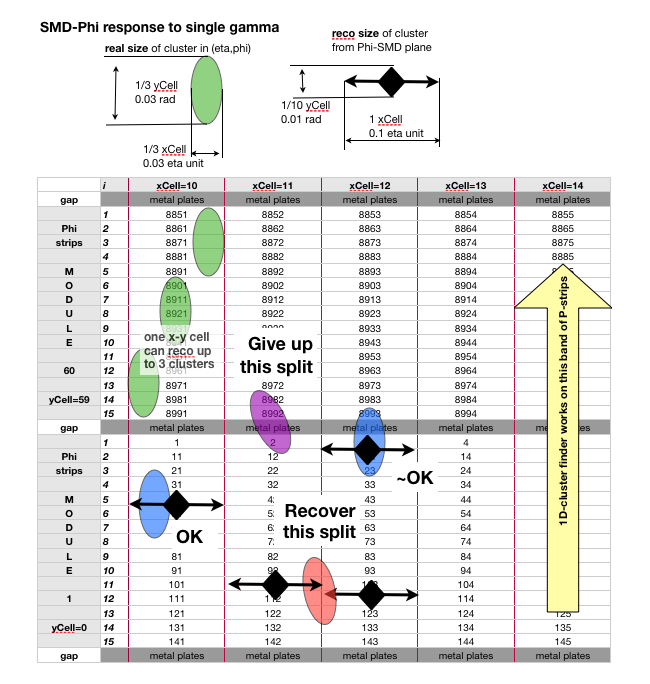
Fig 2.
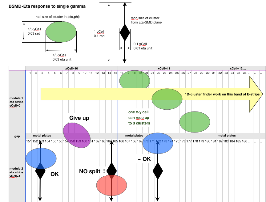
BTOW - Calibration Procedure
Here you will find the calibration procedure for the BTOW (as of 2013).
Additional documentation about BTOW gain calibrations in previous years can be found here:
Report from the STAR EMC Calibrations Workshop (2008)
2006 BEMC Tower Calibration Report
2009 BEMC Tower Calibration Report
As well as in BEMC > Calibrations section on Drupal here.
1) Generating Pedestal/Status Tables
Getting Started
The files which are used for this are from L2 and they're stored on the online "starp" network. You will need to request an account on those machines. Following the instructions here, you should request an account on the "onlldap.starp.bnl.gov" host with the "onlmon" username (you should also request an account with your username if you can). After your request is approved you can log in with the commands shown here:
ssh-agent > agent.sh
source agent.sh
ssh-add
ssh -X -A aohlson@rssh.rhic.bnl.gov  % using your own username, of course
ssh -X -A stargw.starp.bnl.gov
ssh -X -A onlmon@onl05.starp.bnl.gov
It is also necessary to set up the proper directory structure and files.
% after logging in you should be in /ldaphome/onlmon/
mkdir emcstatus2013  % make a directory for the appropriate year
cd emcstatus2013
mkdir pp500  % make a directory for the species/energy
cd pp500
cp ../../emcstatus2012/pp500/l2status.py ./  % copy files from a previous year
cp ../../emcstatus2012/pp500/indexWrite.py ./
cp ../../emcstatus2012/pp500/l2status2012.sqlite3 ./l2status2013.sqlite3
cp ../../emcstatus2012/pp500/empty.sqlite3 ./
cp ../../emcstatus2012/pp500/mapping.sqlite3 ./
cp ../../emcstatus2012/pp500/star_env ./
mkdir db
mkdir db/bemc
mkdir db/eemc
mkdir histoFiles
mkdir /onlineweb/www/emcStatus2013  % make the directories where the online files will be written by indexWrite.py
mkdir /onlineweb/www/emcStatus2013/pp500
mkdir /onlineweb/www/emcStatus2013/pp500/pdf
mkdir /onlineweb/www/emcStatus2013/pp500/details
cd /onlineweb/www
ln -s emcStatus2013 emcStatus  % make a softlink from emcStatus to the current year's directory
cd -
Now you should go through l2status.py and indexWrite.py and change each instance of the year and species/energy to the current ones. Also there are some lines in l2status.py which refer to runnumbers, these should be changed as well. I also like to start fresh with the QA every year, and comment out the lines which hard-code bad channels. The variable "minimumMedianCounts" should be changed to a value appropriate for the species/energy that is being run.
Generating Status/Pedestal Tables with L2
In each run, as part of the L2 algorithm, a 2D histogram is filled with (channel# + 160*crate#) vs. (ADC-l2ped+20). This histogram is named "h22" and is contained within the root files located here: /ldaphome/onlmon/L2algo2013/l2ped/output/ The python macro named "l2status.py" takes this histogram as an input, and generates individual 1D histograms of the ADC spectra for every tower. These histograms are analyzed to determine the tower status, the ADC value of the pedestal peak, and the sigma of the pedestal peak. See below for the status code definitions and examples.
To execute the code do:
source star_env
python l2status.py
You can monitor the progress of the script by looking at l2status.log (for example, by opening another terminal and doing 'tail l2status.log -n50' periodically). As the script progresses you will see the summary pdf files posted to the webpage http://online.star.bnl.gov/emcStatus/pp500/ (for the relevant species/energy), the status and pedestal tables will be written as text files into db/bemc and db/eemc, the actual root histograms will be written into the histoFiles directory, and the results will be written into the database file l2status2013.sqlite3. The statuses and pedestals should be generated once for every good fill.
In a perfect world you would run over the code over the entire dataset once and you would have the status tables which are then uploaded to the STAR database. However, its usually not that simple. There are often problems with a handful of channels that aren't caught by the status checking code, or some that are flagged as bad, but shouldn't be. My suggestion would be to run the code over all the files first and then then we can use the information in the pdfs and in l2status2013.sqlite3 to isolate problem channels. Some of the parameters in the code you may need to tweak to improve the status tables, and some channels you may have to hard code as a bad status for a period of time.
If you want to clear everything and start fresh, you can do this: clean out the folders db/bemc/ and db/eemc/, remove the log file, remove runList.list, and do 'cp empty.sqlite3 l2status2013.sqlite3'
So as a first step, let l2status.py run for a while (it will take time, I often run it in screen so that I don't have to keep a terminal open). You should kill it manually (ctrl+c) when it reaches the end of the runs that you want to look at. When you start it running again it should just pick up (approximately) where it left off.
The code only computes status/pedestal tables if there are enough hits to get good-quality calibrations. The median number of hits above the pedestal must surpass some threshold (minimumMedianHits) in a given fill; this parameter should be set to an appropriate value in l2status.py (not too high that we miss a lot of fills, and not too low that we don't get good calibrations -- there are some examples for appropriate values given in the code). When the threshold is reached you will see some messages in the log file like
2012-06-07 00:26:36 PID: 21394 INFO  medianHits = 635
2012-06-07 00:26:36 PID: 21394 INFO  begin status computation
2012-06-07 00:28:05 PID: 21394 INFO  end status computation -- found 122 bad channels
2012-06-07 00:28:05 PID: 21394 INFO  begin endcap status computation
2012-06-07 00:28:05 PID: 21394 INFO  04TB07 status=136 nonzerohists=22
2012-06-07 00:28:05 PID: 21394 INFO  06TA07 status=136 nonzerohists=18
2012-06-07 00:28:05 PID: 21394 INFO  08TB07 status=136 nonzerohists=21
2012-06-07 00:28:06 PID: 21394 INFO  11TA12 status=0 nonzerohists=60
2012-06-07 00:28:06 PID: 21394 INFO  end status computation -- found 11 bad endcap channels
2012-06-07 00:28:10 PID: 21394 INFO  current state has been saved to disk
2012-06-07 00:28:10 PID: 21394 INFO  creating PostScript file
2012-06-07 00:29:09 PID: 21394 INFO  calling pstopdf
2012-06-07 00:29:42 PID: 21394 INFO  removing ps file
2012-06-07 00:29:43 PID: 21394 INFO  creating endcap PostScript file
2012-06-07 00:29:52 PID: 21394 INFO  calling pstopdf
2012-06-07 00:29:57 PID: 21394 INFO  removing ps file
2012-06-07 00:29:58 PID: 21394 INFO  Finished writing details webpage for  F16732_R13108069_R13108080
2012-06-07 00:30:00 PID: 21394 INFO  goodnight -- going to sleep now
To evaluate the status of each BEMC tower, its ADC spectrum is tested for various features. If a test fails, then a bit (or multiple bits) is flipped to indicate the nature of the problem with the tower. It is possible for a tower to fail multiple tests and therefore have a status code which indicates multiple problems. I show examples of towers which fail each of the basic tests and are therefore assigned specific status codes.
Status Code Definitions
000 == channel does not exist or is masked in L2ped
001 == channel is good
002 == channel is either hot or cold (see bit 16)
004 == channel has a weird pedestal (see bit 32)
008 == channel has a stuck bit (see bits 64 and 128)
016 == if off, hot (10x as many hits); if on, cold tower (10x fewer hits)
032 == if off, pedestal mean is out of bounds; if on, pedestal width is too large/small
064 == bit stuck on
128 == bit stuck off
254 == identical channel
These codes can be seen by going to the EMC Status webpage and clicking on any of the Details pages.
I show examples from a heavy ion (U+U) run where the numbers of counts in the histograms are higher than in p+p, for clarity. All these plots come from the pdf here.
status = 1 (normal ADC spectrum)
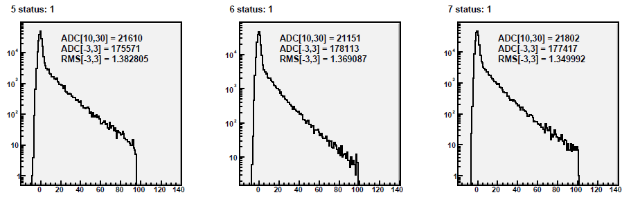
status = 0 (channel is masked out)
Note: MOST of the channels marked with a zero status are (or were) hot channels that were caught and masked out.
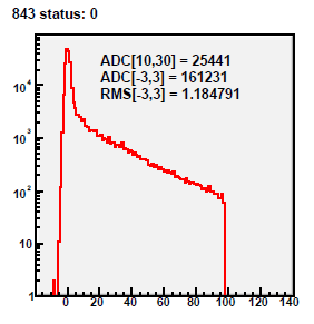
status = 2 (hot channel)
Hot channels look like the above plot, and most of them are caught in realtime and masked out, and thus assigned a status of zero. It is unusual to actually catch a really hot channel after the fact.
status = 18 = 2+16 (cold channel)
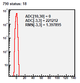
status = 4 or 36 (bad pedestal)
This status catches a range of problems, from weird-looking spectra (like shown here), to wide pedestals, etc.
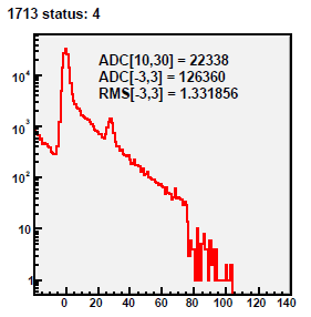
status = 72 = 8+64 (stuck bit - on)
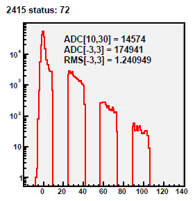
status = 136 = 8+128 (stuck bit - off)
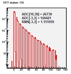
status = 254 (identical channels)
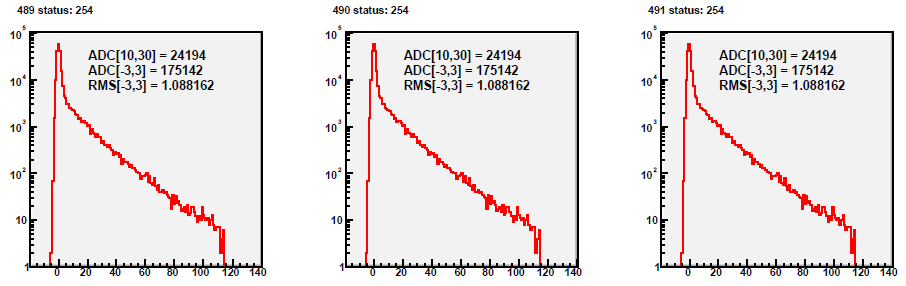
2) QAing the Pedestal/Status Tables
Once the ped/stat tables have been generated, they must be QAed. I do the QA in two parts:
1) I spot check the pdf files by eye. I pick about 5 or 6 fills evenly spaced throughout the run and go through each page of the pdf files looking for any strange-looking towers (for example, towers with stuck bits are pretty easy to see, and they don't always get caught by the algorithm). Yes, this takes a while, but we don't have to look at the pdfs for every fill!
For examples of the bad channels you are looking for, have a look at Suvarna's nice QA of the tables last year:
https://drupal.star.bnl.gov/STAR/blog/sra233/2012/dec/05/bemc-statuscuau200hard-coded-towers
https://drupal.star.bnl.gov/STAR/blog/sra233/2012/aug/15/bemc-statuspp200towers-with-status-marked-oscillating
2) The status and pedestal information is stored in the sqlite database file, and we can spin over this quickly in order to look at the data over many runs/fills. I have attached a script which is used to analyze the database file l2status2013.sqlite3. The first step is to download l2status2013.sqlite3 somewhere *locally* where you can look at it, and save statusCheckfill2.py in the same place. In statusCheckfill2.py you should change line 27 to the appropriate run range that you are analyzing, and change 2012-->2013 if necessary. Then all you need to do to run the code is something like:
setenv PYTHONPATH $ROOTSYS/lib
python statusCheckfill2.py
This python code allows you to look at the statuses and pedestals from run to run. At the moment I make lists of the statuses and pedestals for each tower (in the variables u and y -- sorry for my horrible naming scheme!), and then I can print these lists to the screen or graph them. At the moment I have the code so that it prints the statuses for any tower that has status 1 some, but not all, of the time (line 138). This script can be used to find channels which change status frequently over the course of the run... for example, sometimes there are channels which are right on the edge of satisfying the criteria for being marked as "cold" and therefore their status alternates 1 18 1 1 18 18 1 1 18 1 18 etc. Then we can look at the pdf files to see if the tower always looks cold, or if its behavior really changes frequently. If it is truly cold, then at that point we can either adjust the criteria for being marked as cold, or hard-code the channel as status 18 (I typically just hard-code it).
Also I can look at the histograms histoPedRatio and histoPedRatioGood (which are saved out in histogramBEMCfill.root), which are plots of the ratio of the pedestal for a given run to the pedestal of the first run as a function of tower id. histoPedRatio is filled for every tower for every run (unless the pedestal for that tower in the first run is zero), and histoPedRatioGood is only filled if the tower's status is 1. I haven't needed to cut out any towers based on these plots, but I think they would be a good way to find any towers whose pedestals are fluctuating wildly over time (or maybe you might want want to plot the difference, not the ratio).
So you can take a look at the code and play around with it so that it allows you to do the QA that you think is best.
If you look at l2status.py, you can see where I've hard-coded a bunch of channels I thought were bad (the lines which hard-code bad channels are commented out right now because I prefer to start from scratch each year). I've pasted the code here too:
## hard code few bad/hot channels
#if int(tower.softId)==939 : ##hard code hot channel
# tower.status |= 2
#if (int(tower.softId)==3481 or int(tower.softId)==3737) : ##hard code wide ped
# tower.status |= 36
#if (int(tower.softId)==220 or int(tower.softId)==2415 or int(tower.softId)==1612 or int(tower.softId)==4059): ##hard code stuck bit
# tower.status |= 72
if (int(tower.softId)==671 or int(tower.softId)==1612 or int(tower.softId)==2415 or int(tower.softId)==4059) : ##hard code stuck bit (not sure which bit, or stuck on/off)
tower.status |= 8
if (int(self.currentFill) > 16664 and (int(tower.softId)==1957 or int(tower.softId)==1958 or int(tower.softId)==1977 or int(tower.softId)==1978 or int(tower.softId)==1979 or int(tower.softId)==1980 or int(tower.softId)==1997 or int(tower.softId)==1998 or int(tower.softId)==1999 or int(tower.softId)==2000 or int(tower.softId)==2017 or int(tower.softId)==2018 or int(tower.softId)==2019 or int(tower.softId)==2020)) : ##hard code stuck bit
tower.status |= 8
if (int(tower.softId)==410 or int(tower.softId)==504 or int(tower.softId)==939 or int(tower.softId)==1221 or int(tower.softId)==1409 or int(tower.softId)==1567 or int(tower.softId)==2092) : ##hard code cold channel
tower.status |= 18
if (int(tower.softId)==875 or int(tower.softId)==2305 or int(tower.softId)==2822 or int(tower.softId)==3668 or int(tower.softId)==629 or int(tower.softId)==2969 or int(tower.softId)==4006) : ##either cold or otherwise looks weird
tower.status |= 18
Some of these channels are persistently problematic, so I expect that your list of bad channels will look similar to mine from previous years.
It may take a few iterations of generating the tables, finding bad towers, tweaking the code or hard-coding the bad channels, regenerating the tables, etc before you are satisfied with the quality of the tables. Once you have run l2status.py one last time and are satisfied with the quality of the tables you have generated, they are ready to be uploaded to the database by the software coordinator.
3) Uploading Pedestal/Status Tables to the Database
Once the ped/stat tables have been QAed satisfactorily, the values need to be uploaded to the database.
First, the files in /db/bemc/ need to be moved to RCF, where the upload will take place. This can be done with the following commands:
ssh-agent > agent.sh
source agent.sh
ssh-add
ssh -X -A aohlson@rssh.rhic.bnl.gov % using your own username
rterm -i
mkdir bemcUpload2013 % make a directory to work in
mkdir bemcUpload2013/tables
cd bemcUpload2013/tables/
scp onlmon@onl05.starp.bnl.gov:'/ldaphome/onlmon/emcstatus2013/pp500/db/bemc/*.txt' ./
cd ../
The scripts bemcPedTxtUpload.C and bemcStatTxtUpload.C are used to perform the upload. They take as input the name of a file which contains a list of the files to be uploaded. To create the file lists:
% in bemcUpload2013/
mkdir lists
cd tables
ls bemcStatus*.txt > ../lists/bemcStatus.list
ls bemcPed*.txt > ../lists/bemcPed.list
cd ../
Once the file lists have been created, the scripts can be run with:
stardev
setenv DB_ACCESS_MODE write
root4star bemcStatTxtUpload.C
root4star bemcPedTxtUpload.C
Important!
1) The upload scripts (bemc*TxtUpload.C) contain return statements to prevent accidental uploads. Make sure everything is working properly by running the scripts with the return statements included (nothing will be uploaded to the db) first. When you are sure that you're ready to upload, then comment out the return statements. After uploading, don't forget to uncomment the return statements!
2) Try uploading one table first, and then check that it is uploaded correctly (see below), before uploading all the tables for the whole run. If a table is uploaded wrongly, it can be disactivated by the software team, but this is not something we want to do often. (In the case of a single table, it may be more efficient to just upload the correct table with a timestamp one second after the incorrect table.)
3) Reminder: this is not a task many people should need to do but should be limited to one or two "experts", who will be given special DB writing priviledges by Dmitry Arkhipkin (arkhipkin@bnl.gov).
Uploaded tables can be viewed with the online BEMC DB browser. I find it helpful to spot-check some tables to make sure they have been uploaded correctly. I find a table with the browser, copy it into an text file, and compare it to the text file I uploaded (in tables/). For the status tables, this can be done with a simple diff command. For the pedestal tables, the script checkPeds.C can be used.
At the beginning of the run (after physics has been declared, L2 is running, etc), it is good to generate a set of ped/stat tables and upload them to the database one second after the initialized values (for example, at 20131220.000001). (Reminder: The procedure for initializing the timeline with ideal values can be found here.) This can be done with the bemc*TxtUpload.C scripts; you will see a commented-out line that shows how to set the timestamp manually. It is good to do this periodically throughout the run, especially if something changes with the detector or beam configuration, so that FastOffline reconstruction can pick up decent DB values. Each time, the tables should be uploaded one second after the previous tables, so that when we upload the fully-QAed tables at the end of the run, the temporary ones will no longer be picked up.
4) Relative Gain Calibration with MIPs
Getting Started
1) The code needed to perform the gain calibrations can be checked out from CVS and compiled. In your working directory, do:
 cvs co StRoot/StEmcPool/StEmcOfflineCalibrationMaker/
cons
You can move the required files to your working directory, or make soft links. You need the following files, which are in the macros/ directory:
-- bemcCalibMacro.C
-- btow_mapping.20030401.0.txt
-- CalibrationHelperFunctions.cxx
-- CalibrationHelperFunctions.h
-- electron_drawfits.C
-- electron_histogram_maker.C
-- electron_master.C
-- electron_master_alt.C
-- electron_tree_maker.C
-- geant_fits.root
-- mip_histogram_fitter.C
-- mip_histogram_maker.C
-- SubmitCalibJobs.pl
-- runMIPjobs.sh
-- runElecJobs.sh
-- runFinalElecJobs.sh
Some of the files have lists of triggers which need to be hard-coded in for each year. In particular, in bemcCalibrationMacro.C you should ensure that the correct trigger list is present, and the trigger IDs for the HT triggers need to be written in StEmcOfflineCalibrationMaker.cxx. (In most cases I have already typed in the values for Run 11, but they are commented out while the Run 9 values are commented in.) If you want to use the TOF information (in Run 11 and beyond), there are some lines of code that need to be commented in in StEmcOfflineCalibrationMaker.cxx.
Generating Trees
2) Generate the list of runs with the following command (for Run 9)
get_file_list.pl -keys "runnumber" -distinct -cond "production=P11id,filetype=daq_reco_MuDst,sanity=1,trgsetupname=production2009_200GeV_Single,filename~st_physics,tpx=1,emc=1,storage!=HPSS" -limit 0 | sort -u > runlist.txt
or similar for other years.
3) Run SubmitCalibJobs.pl, which will execute the bemcCalibMacro.C macro. Make sure that the correct catalog query lines are commented in/out in the submit script. Also ensure that the appropriate directories exist ($workingDir, $schedDir, $outDir, $logDir, $scriptDir) as specified at the top of the submit script.
This macro creates trees which store primary tracks which will be further analyzed for the calibration. For each primary track we write out the track information from the TPC, the EMC information for the 3x3 tower cluster around the track, the TOF information (in Run 11 and beyond), and the trigger information.
The trees created by this step are stored on HPSS here:
Run 9: /home/aohlson/bemcCalib2009_x.tar where x=0,...,9
Run 11: /home/aohlson/bemcCalib2011_05_x.tar where x=0,...,14 and /home/aohlson/bemcCalib2011_07_x.tar where x=0,...,18
MIP calibration
The relative gain calibration is obtained by finding the MIP peak in each of the 4800 BEMC towers.
The MIP energy deposit has the following functional form, which was determined from test beam data and simulations:
MIP = (264 MeV)×(1+0.056η2)/sin(θ)
From this expression we can calculate a calibration constant
C = 0.264×(1+0.056η2)/(ADCMIP×sin(θ))
where ADCMIP is the location of the MIP peak in the ADC spectrum. This allows us to combine towers at the same η and thus find the absolute gain calibration in each crate-slice using electrons (see next section).
The procedure for obtaining the MIP calibration is as follows...
4) Make the MIP histograms with runMIPjobs.sh which executes mip_histogram_maker.C Ensure that the correct output filenames are specified in the submit script.
Events with |vz| < 30 cm are selected, and any towers that have multiple tracks associated with them are excluded. We select tracks with p > 1 GeV/c, and require that they enter and exit the same tower. We require that the towers surrounding the central tower do not contain a large energy deposition. We require that ADC-ped > 1.5*pedRMS. After these track quality cuts we fill histograms with the ADC-ped values for each tower.
5) Make a list of the output files from step (4) called mips.list. Run mip_histogram_fitter.C
We fit each histogram with a gaussian on a pedestal; the histograms and fits are shown in mip.pdf. If the fit values fail basic quality cuts (such as if the mean is < 5), then the tower is assigned a bad status (!=1). These fits are marked as red in mip.pdf. For each tower we record the mean and sigma of the gaussian fit, and the status.
6) Check mip.pdf by eye to look for any other towers which were obviously bad. Write a function like isBadTower2009(int id) (see examples in the code) which identifies these bad towers so that they can be assigned a bad status. You can either put this function in mip_histogram_fitter and re-run it, or you can put it in the electron codes. Note that most of the towers with bad MIP peaks were marked as bad (cold/hot/stuck bit) towers when the status/pedestal tables were originally computed.
5) Absolute Gain Calibration with Electrons
Electron calibration
The absolute gain calibration is done by identifying electrons and finding the E/p peak for small groupings of towers. It is desirable to find the E/p peak for as small groupings as possible. In 2006 the calibration was done in rings in η, while in 2009 it was done for "crate-slices", which are groups of 8 towers in the same crate in the same η ring.
The procedure is as follows...
7) Make the electron trees with runElecJobs.sh which will execute electron_tree_maker.C Ensure that the correct output filenames are specified in the submit script.
The macro electron_tree_maker.C makes slimmer trees of electron candidates which satisfy the following criteria:
-- event vertex |vz| < 60
-- track must come from reconstructed vertex (ranking >= 0)
-- 1.5 < p < 20 GeV/c
-- nhits >= 10
-- matched tower status = 1
-- dE/dx > 3e-6
-- ADC-ped > 1.5*pedRMS
In this macro, if the electron track points towards a HT trigger tower then it is assigned htTrig = 2
8)
In the old calibration: Make a list of the output files from step (5) called electrons.list. Run electron_master.C.
---- OR ----
In the new calibration: Run runFinalElec.sh, which executes electron_master_alt.C (make sure that the input/output filenames and directories are correct). Hadd the resulting output files, and use this file as the input to electron_drawfits.C
In this macro even more stringent cuts are placed on the electron candidates:
-- ADC-ped > 2.5*pedRMS
-- track must enter and exit the same tower
-- p < 6 GeV/c
-- track does not point towards a tower which fired the HT trigger (htTrig != 2)
-- dR < 0.025 (distance from the center of the tower)
-- dE/dx > 3.4e-6
-- the maximum Et in the 3x3 cluster of towers must be in the central tower
-- there are no other tracks pointing to the central tower
The resulting histograms of E/p in each crate-slice are drawn and fit with a Gaussian plus a first-order polynomial. If the calibration is already correct, then the E/p peak should be at 1. The deviation from unity establishes the absolute gain calibration which, combined with the relative gain calibration from the MIP procedure, defines the overall BEMC gain calibration.
Run 12 BTOW Calibration
This is parent page that will hold all informationa about the run12 BEMC gain calibration
200 GeV Calibration
This calibration was done with the 200 GeV proton-proton data collected in 2012. The calibration trees are backed up on HPSS and can be found here:
/home/jkadkins/bemcCalibrations/2012/pp200/bemcCaibTrees2012-0XX.tar
where XX = 0, 1, 2, .... , 34
Run 3 BTOW Calibration
I plan on "Drupalizing" these pages soon, but for now here are links to Marco's slope calibration and Alex's MIP and Electron calibrations for the 2003 run:
Marco's tower slope calibrationAlex's MIP calibration
Alex's electron normalization
Run 4 BTOW Calibration
Introduction:
The recalibration of the BEMC towers for Run 4 includes the following improvements:
- recovery of 158 swapped towers
- identification and removal of 38 towers with possible light leakage / electronics problems
- identification and removal of 24 towers with bad p/E distributions
- MIP calibration restricted to low-multiplicity events from minimum-bias data
- isolation requirement imposed on MIP candidates

Notes:
- p0 * 4066 = 28.5 GeV full-scale at zero rapidity (assuming pedestal~30).
- 2191/2400 = 91.3% of the towers have nonzero gains.
- Despite the differences in the cuts used, the final gains are similar to the ones currently found in the DB; a histogram of (newgain-dbgain)/newgain for the towers present in both calibrations yields a mean of 0.019 and an rms of 0.03896.
Procedure:
The offline calibration of the BEMC towers for Run 4 is accomplished in three steps. In the first step, MIPs are collected for each tower and their pedestal-subtracted ADC spectra are plotted. The MPV of the distribution for each tower is translated into a gain using an equation originally established by test-beam data (SN 0433). In the second step, electrons are collected for each eta-ring and the ratio of their momentum and energy (with the energy calculated using the MIP gains from step 1) is plotted as a function of the distance between the track and the center of the tower. The calculated curve is fit to a GEANT simulation curve, allowing extraction of scale factors for the MIP gains in each eta ring. Finally, all electrons in all eta-rings are grouped together and the ratio of their energy and momentum (E/p) is plotted, with the energy calculated from the rescaled gains in the second step. The distribution is fit with a Gaussian and a scale factor is applied so that this Gaussian is centered exactly on 1.000.
Catalog query:
<inputURL="catalog:star.bnl.gov?production=P05ia||P05ib||P05ic,sanity=1,tpc=1,emc=1, trgsetupname=ProductionMinBias||productionLow||productionMid||productionHigh,filename~physics, filetype=daq_reco_mudst,magscale~FullField,storage!~HPSS,runnumber>=5028057" nFiles="all" />
Working directories:
/star/u/kocolosk/emc/offline_tower_calibration/2004/jan25_2004mip/
/star/u/kocolosk/emc/offline_tower_calibration/2004/jan30_2004electron/
MIP Cuts:
- track momentum > 1
- track enters, exits same tower
- 1 track / tower
- (ADC - ped) > 2*pedRMS
- trigger == 15007 (mb data)
- abs(z-vertex) < 30
- reference multiplicity < 57 (60-100% centrality)
- isolation cut (all neighboring towers satisfy (ADC-ped) < 2*pedRMS)
Electron Cuts:
- 1.5 < track momentum < 20
- track enters, exits same tower
- 1 track / tower
- # track points > 25
- 3.5 < dEdx < 4.5 keV/cm
- (ADC - ped) > 2*pedRMS
- trigger != 15203 (excludes most ht-triggered electrons; should have been trigger == 15007 to get mb-only data)
Adam Kocoloski, 14 Feb 2006
Run 5 BTOW Calibration
Introduction
The final BTOW calibration for Run 5 offers the following improvements over previous database calibrations:
- recovery of 194 swapped towers
- identification and exclusion of 51 towers with correlated firing problems
- identification and exclusion of 33 towers with p/E~0.6
- exclusion of 58 towers with PMTs replaced by Stephen and Oleg during the shutdown
- isolation cut removes background from MIP spectra, identifies correlated towers
- 30 cm vertex cut introduced to reduce path length differences among MIPs
- uniform scale factor (1.04613) introduced after eta ring electron normalization to set E/p==1 when integrated over all towers


p0 = 0.00696912 for the fit parameter implies an <ET> = 28.3 GeV on the west side, but the gains do not seem to be well described by the 1/sin(theta) fit
3997/4240 = 94.3% of commissioned towers have nonzero gains
Procedure
The offline calibration of the BEMC towers for Run 5 is accomplished in three steps. In the first step, MIPs are collected for each tower and their pedestal-subtracted ADC spectra are plotted. The MPV of the distribution for each tower is translated into a gain using an equation originally established by test-beam data (SN 0433). In the second step, electrons are collected for each eta-ring and the ratio of their momentum and energy (with the energy calculated using the MIP gains from step 1) is plotted as a function of the distance between the track and the center of the tower. The calculated curve is fit to a GEANT simulation curve, allowing extraction of scale factors for the MIP gains in each eta ring. Finally, electrons in all eta-rings that pass through the center of a tower are grouped together and the ratio of their energy and momentum (E/p) is plotted, using the energy calculated from the rescaled gains in the second step. The ditribution is fit with a Gaussian and a scale factor is applied so that this Gaussian is centered exactly on 1.000.
Catalog query:
<input URL="catalog:star.bnl.gov?production=P05if,tpc=1,emc=1, trgsetupname=ppProduction||ppTransProduction||ppProductionMinBias, filename~st_physics,filetype=daq_reco_mudst,storage!~HPSS" nFiles="all" />Working directories:
/star/u/kocolosk/emc/offline_tower_calibration/2005/feb08_2005/
/star/u/kocolosk/emc/offline_tower_calibration/2005/feb08_earlyfiles/
The 2005 directory contains jobs run using Dave Relyea's offline pedestals (the bulk of the data), while the earlyfiles directory uses online pedestals for runs before April 26th that are not included in the offline pedestal calculations.
MIP Cuts:
- track momentum > 1
- track enters, exits same tower
- 1 track / tower
- (ADC - ped) > 2*pedRMS
- abs(z-vertex) < 30
- isolation cut (all neighboring towers satisfy (ADC-ped) < 2*pedRMS)
- no trigger selection (previous statement of mb-only triggers was in error)
Electron Cuts:
- 1.5 < track momentum < 20
- track enters, exits same tower
- 1 track / tower
- # track points > 25
- 3.5 < dEdx < 4.5 keV/cm
- (ADC - ped) > 2*pedRMS
- no trigger selection
For More Information:
Detailed information on this and other BTOW calibrations, including tower-by-tower MIP and p/E spectra and a summary of outstanding issues, is available at
http://www.star.bnl.gov/protected/spin/kocolosk/barrel_calibration/saved_tables/
The calibration summarized here has the timestamp 20050101.000001.
First Calibration using CuCu data
Runs used: 6013134 (13 Jan) - 6081062 (22 Mar)
The procedure for performing the relative calibration can be divided into 3 steps:
- Create a histogram of the pedestal-subtracted ADC values for minimum-ionizing particles in each tower
- Identify the working towers (those with a clearly identifiable MIP-peak)
- Use the peak of each histogram together with the location of the tower in eta to calculate a new gain
- Create new gain tables and rerun the data, this time looking for electrons
- Use the electrons to establish an absolute energy scale for each eta-ring
Using Mike's code from the calibration of the 2004 data, an executable was created to run over the 62GeV CuCu data from Run 5, produce the 2400 histograms, and calculate a new gain for each tower. It was necessary to check these histograms by hand to identify the working towers. The output of the executable is available as a 200 page PDF file:
2005_mip_spec.pdf (2400 towers - 21.6 MB)
Towers marked red or yellow are excluded from the calibration. Condensed PDFs of the excluded towers are available at the bottom of the page ("bad" and "weird"). In all, we have included 2212 / 2400 = 92% of the towers in the calibration.
Systematic Behavior of the Gains
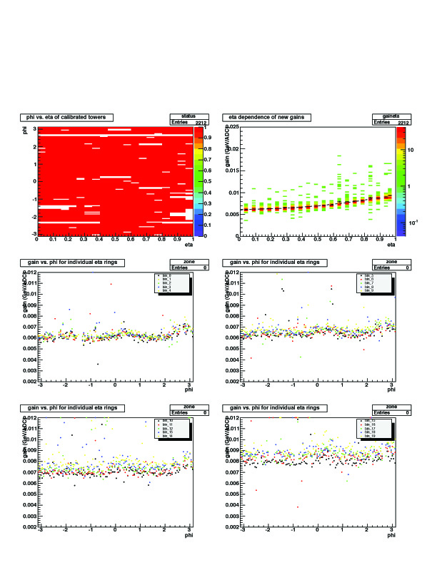
The first plot in the top left shows the excluded towers (white blocks) in eta_phi space
In the second plot we collect the towers into 20 eta-rings (delta-eta = 0.05) and look at the change in gain as we move out in eta. This plot shows the expected increase in gain as we move into the forward region (except for eta-rings 19 and 20).
Finally we look at each individual eta-ring for for systematic variations in azimuth. There appears to be some structure around phi=0.2 and phi=3.
Electron Calibration Status
We have made an attempt to realize the absolute energy scales using electrons. Unfortunately, there does not appear to be a sufficient number of electrons in the processed 62GeV data to do this for each eta-ring. We will revisit this later when more statistics are available, but in the meantime we have established the following workaround:
- Fit the average gains of the first 17 eta-rings with a function that goes as 1/sin(theta)
- Caclulate the expected gains for eta-rings 18, 19, and 20 from this function
- Scale the forward eta-rings accordingly
The results of this procedure are seen in an updated plot of gain vs. eta:
Here are new bemcCalib and bemcStatus .root files created using these rescaled gains:
bemcCalib.20050113.053235.root
bemcStatus.20050113.053235.root
The text file is a list of tower-gain pairs. A gain of zero indicates a tower that has been masked out. Finally, we have a plot of p/E summed over all eta:

Update: Addition of the East BEMC Towers
We have calculated new gains for the 1200 towers in the east half of the barrel that were turned on by March 22. Only data from March 22 were used in this calibration. The results can be found in 2005_mip_spec_newtowers.pdf
bemcCalib.20050322.000000.root
bemcStatus.20050322.000000.root
The gains for towers 1-2400 are the same as before. These files include those entries, as well as new gains for towers 2401-4800. No attempt has been made to get an absolute energy scale for the east towers, so we still see the drop in gain for large eta:

Implementation of Tower Isolation Cut
Originally posted 11 October 2005
Previously we had calibrated the BEMC using data from all triggers. We now have enough data to restrict ourselves to minimum-bias triggers. Additionally, we have implemented a cut that requires the pedestal-subtracted ADC value of neighboring towers to be less than twice the width of the pedestal. This cut does an excellent job of removing background, especially in the high-eta region:
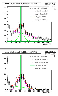
The cut is used in the bottom plot. Unfortunately there is also a small subset of towers where the isolation cut breaks the calibration:
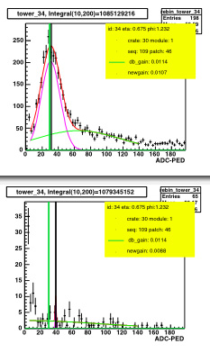
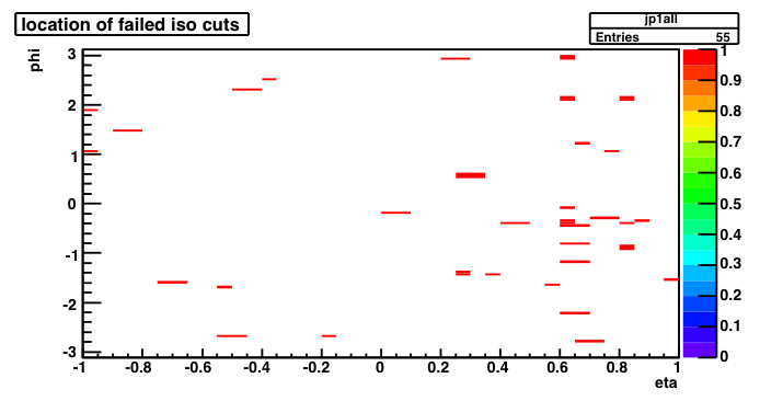
Again the cut is used in the bottom plot. We have decided to use the isolation cut when possible, and use the full minimum-bias data in the case of the (55) towers for which the cut breaks the calibration. This new calibration is able to recover ~30 towers that were previously too noisy to calibrate. We are in the process of reviewing the remaining bad towers found in 2005_MinBiasBadTowers.pdf. Towers 671,1612, and 4672 appear to have problems with stuck bits in the electronics, and there are a few other strange towers, but the majority of these towers just seem to have gains that are far too high. We plan on reviewing the HV settings for these towers. An ASCII file of the bad towers is attached below.
Recalibration Using pp data
Originally posted 26 September 2005
Catalog query:
input URL="catalog:star.bnl.gov?production=P05if,tpc=1,emc=1,trgsetupname=ppProduction,filename~st_physics,filetype=daq_reco_mudst,storage=NFS" nFiles="all"
note: 3915/4240 = 92.3% of the available towers were able to be used in the calibration. Lists of bad/weird towers in the pp run are available by tower id:
bad_towers_20050914.txt
weirdtowers_20050914.txt
The relative calibration procedure for pp data is identical to the procedure we used to calibrate the barrel with CuCu data (described below). The difference between pp and CuCu lies in the electron calibration. In the pp data we were able to collect enough electrons on the west side to get an absolute calibration. On the east side we used the procedure that we had done for the west side in CuCu. We used a function that goes like 1/sin(theta) to fit the first 17 eta rings, extrapolated this function to the last three eta rings, and calculated the scale factors that we should get in that region. Here is a summary plot comparing the cucu and pp calibrations for the 2005 run:

Comparing the first two plots, one notices immediately that many of the pp gains on the east (eta < 0) side are quite high. A glance at the last plot on the summary canvas reveals a collection of towers with phi < -pi/2 that have unusually high gains. These towers were added during the pp run and hence their gains are based on nominal HV values without any iteration (thanks Mike, Stephen). If we mask out those towers in the summary plot, the plots look much more balanced:

The bottom plot clearly shows that the final pp gains are ~10% higher than the gains established from the mip calibration using the cucu data. Moreover, the cucu data closely follows a 1/sin(theta) curve, while the curve through the pp data is flatter. This is revealed in the shape of the bottom plot. Note that we never scaled the gains near eta=-1 for the cucu data, which is why there is still a significant drop-off in the ratio of the mean gains in that region.
New calibration and status tables (including the gains for the new towers that were turned on during pp running) are available at
bemcCalib.20050322.000001.root
bemcStatus.20050322.000001.root
It should be noted that the scale factors we used to get the final gains near eta=-1 on the east side were calculated without the new towers since they were throwing off the fit function. However, those new towers still had their final gains scaled before we produced the calibration and status tables.
Systematic Uncertainty Studies
In the 2003+2004 jet cross section and A_LL paper we quoted a 5% systematic uncertainty on the absolute BTOW calibration. For the 2005 jet A_LL paper there is some interest in reducing the size of this systematic.I went back to the electron ntuple used to set the absolute gains and started making some additional plots. Here's an investigation of E_{tower} / p_{track} versus track momentum. I only included tracks passing directly through the center of the tower (R<0.003) where the correction from shower leakage is effectively zero.
Full set of electron cuts (overall momentum acceptance 1.5 < p < 20.):
dedx>3.5 && dedx<4.5 && status==1 && np>25 && adc>2*rms && r<0.003 && id<2401
I forgot to impose a vertex constraint on these posted plots, but when I did require |vz| < 30 the central values didn't really move at all.
Here are the individual slices in track momentum used to obtain the points on that plot:

Electrons with momentum up to 20 GeV were accepted in the original sample, but there are only ~300 of them above 6 GeV and the distribution is actually rather ugly. Integrating over the full momentum range yields a E/p measurement of 0.9978 +- 0.0023, but as you can see the contributions from invididual momentum slices scatter around 1.0 by as much as 4.5%
Next Steps? -- I'm thinking of slicing versus eta and maybe R (distance from center of tower).
Run 6 BTOW Calibration
Introduction
This is not the final calibration for the 2006 data, but it's a big improvement over what's currently in the DB. It uses MIPs to set relative gains for the towers in an eta ring, and then the absolute scale is set by electron E/p.
Isolation Cut Failures
This is a problem that we encountered in 2005, where several pairs of towers had good-looking spectra until the isolation cut was applied, and then quickly lost all their counts. Well, all of the towers that I had tagged with this problem in 2005 still have it in 2006, with one exception. Towers 1897 and 1898 seem to have miraculously recovered, and now towers 1877 and 1878 appear to have isolation failures. Perhaps this is a clue to the source of the isolation failures?
Dataset:
everything I could find on nov07:
<input URL="catalog:star.bnl.gov?production=P06ie,sanity=1,tpc=1,emc=1,trgsetupname= ppProduction||ppProductionTrans||ppProductionLong||pp2006MinBias||ppProductionJPsi||ppProduction62||ppProductionMB62, filename~st_physics,filetype=daq_reco_mudst" nFiles="all" />
Cuts:
Same as 2005. All MIP fits are basic Gaussians over the range 5..250 ADC-PED. Electron fits are Gaussian + linear in a very crude attempt to estimate hadronic background.
Working Directory:
/star/u/kocolosk/emc/offline_tower_calibration/2006/nov07/
Plots:
The gains look pretty balanced on the east side and west side. Note that I didn't multiply by sin(theta), so we expect an eta-dependence here. The widths plot is interesting because it picks out one very badly behaved crate on the east side at phi=0. I believe it is 0x0C, EC24E (towers 4020-4180). The tower fits are attached below if you're interested. Bad towers are marked in red.

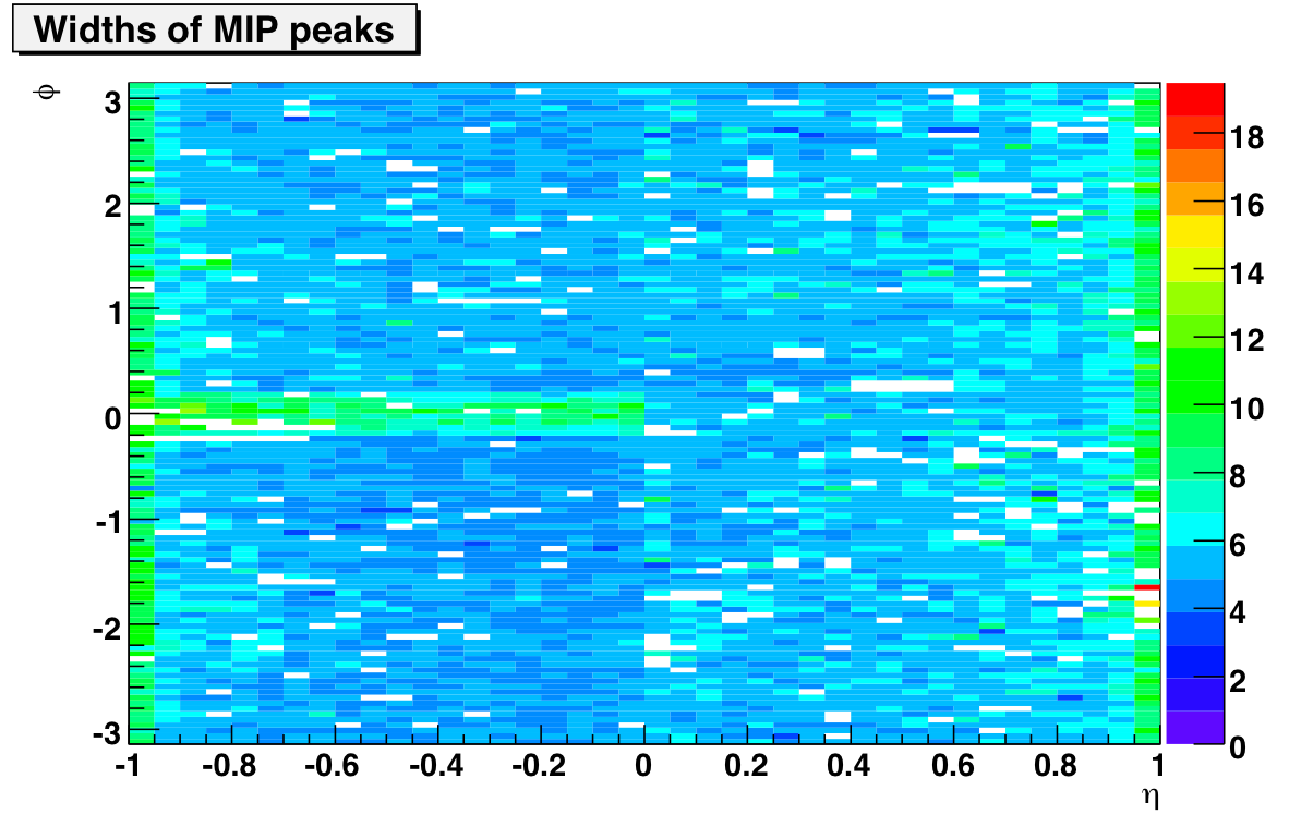
Electron Normalization:
E/p plots for all 40 eta-rings (first 20 on west side, 21-40 on east side) are attached below. In general, the electrons indicate a 9-10% increase in the MIP gains is appropriate. In the last two eta rings on each side, that number jumps to 20% and 40%. This is more or less consistent with the scale factors found in the 2003 calibration (the last time we used a full-scale energy of 60 GeV. If I scale the MIP gains and plot the full-scale E_T I get the plot on the left. Fitting the eta dependence with a pol0 over the middle 36 eta rings results in a ~62 GeV scale and a nasty chi2.
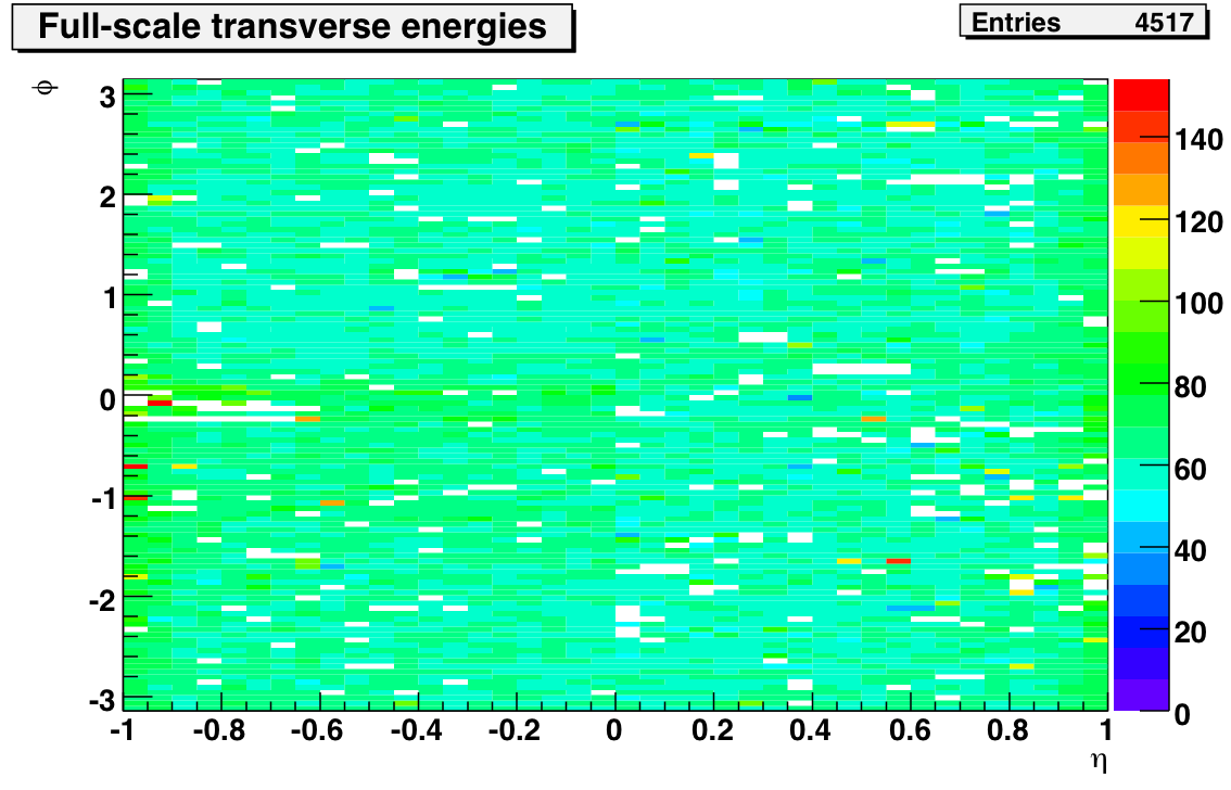
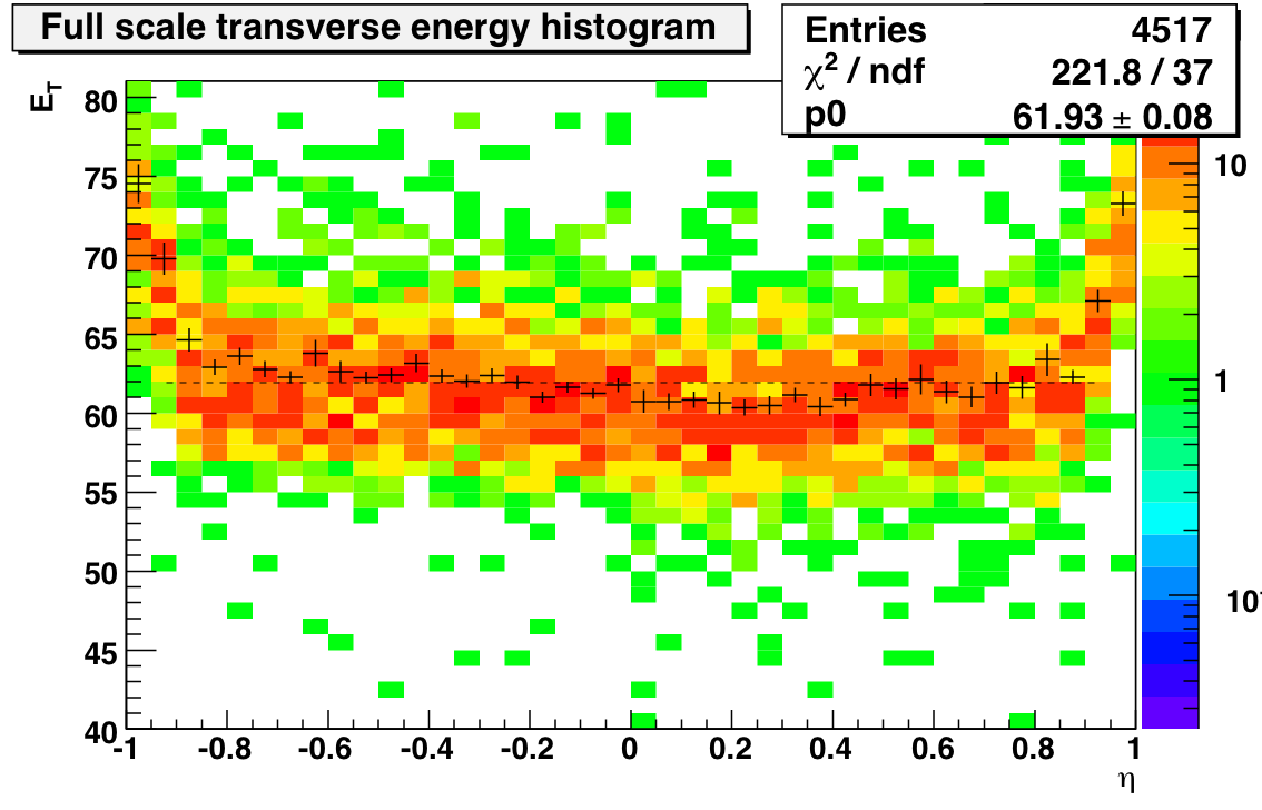
So after scaling with the electrons it looks like we are actually a couple of GeV high on the absolute scale. I'll see if this holds up once I've made the background treatment a little more sophisticated there. I also have to figure out what went wrong with the electrons out at the edges. I didn't E/p would be that sensitive to the extra material out there, but for some reason the normalization factors out there are far too large. Next step will be to comapre this calibration to one using electrons exclusively.
Calibration Uncertainty:
Here are some links that address different parts of the calibration uncertainty that are not linked from this page:
drupal.star.bnl.gov/STAR/subsys/bemc/calibrations/run6/btow/calibration-uncertainty-calculation
drupal.star.bnl.gov/STAR/blog-entry/mattheww/2009/apr/09/2006-calibration-uncertainty
drupal.star.bnl.gov/STAR/blog-entry/mattheww/2009/apr/27/crate-systematic-2006
Online Work
Steve's caiibrations page contains most of the details:http://www.star.bnl.gov/protected/spin/trent/calibration/calibration.html
Some files of slopes, etc. that I produced are currently stored at
http://web.mit.edu/kocolosk/www/slopes/
MIP check on 2006 Slope Calibration
~300k events processed using fastOffline:
Run 7079034 ~189K
Run 7079035 ~115K
Number of events with nonzero primary tracks = 109k / 309k = 35%
Still a few problems with pedestal widths in the database, although now they appear to be restricted to id > 4200. If I don't cut on adc>2*rms, the software id distribution of MIPs looks pretty isotropic:
The distribution of primary tracks also looks a lot better:
I was able to calculate MIP gains for each of the 40 eta-rings. The plot at the top fits a line to the full-scale transverse energies extracted from the gains (excluding the outer two eta-rings on each side). For the error calculations I used the error on the extraction of the mean of the MIP ADC peak and propagated this through the calculation. This is not exactly correct, but it's a pretty close approximation. In a couple of cases the error was exceedingly small (10^-5 ADC counts), so I forced it to an error of 1 GeV (the fit failed if I didn't).
As you can see in the text file, an error of 1 ADC in the MIP peak leads to an error of 3 GeV in the full-scale transverse energy. Therefore I would say that pedestal fluctuations (1-2 ADCs) give an additional error of 5 GeV to my calculations, which means that the majority of these eta-rings are consistent with a 60 GeV full-scale.
Conclusions:
- A straight-line fit yields 56 GeV as the average full-scale transverse energy of the towers
- We have enough stats; errors are dominated by pedestal fluctuations leading to a 5 GeV uncertainty
- Tower response is flat in E_t across eta-rings (excluding last two rings where MIPs fail)
- Good job Stephen and Oleg!
The First Attempt
Note: The first attempt at this analysis was plagued by poor TPC tracking and also problems with corrupted BTOW pedestal widths in the database. I'm including the content of the original page here just to document those problems.
250k events processed using fastOffline:
Run 7069023 100K
Run 7069024 100K
Run 7069025 50K
Number of events with nGlobalTracks > 0 = 30166 (12%)
On the left you see the software id distribution of slope candidates (adc-ped>3*rms, no tracking cuts). There's a sharp cutoff at id==1800. But before you go blaming the BEMC for the missing MIPs, the plot on the right shows eta-phi distribution of global tracks without any EMC coincidence. The hot region in red corresponds to 0<id<1800:
As it turns out, the missing slope candidates are likely due to wide pedestals. The pedestal values look fine, but if I plot pedrms for id<1800 and id>1800 using the slope candidates that did survive:
Is it possible that the TPC track distribution is connected to this problem?
2006 Gain uniformity
Using the gains we calculated for 2006 tower by tower from the MIPs and then corrected with the electron eta rings, I calculated how it differed from the ideal gain assuming containment of an EM shower with 60 GeV ET. After removing bad towers, we can fit the distribution of this ratio to a gaussian and we find there is approximately a 6% variation in the gains.


Calibration Uncertainty Calculation
Summary:
The uncertainty on the 2006 BTOW Calibration is 1.6%. This value is the combination of a 1.3% overall uncertainty and a 0.9% uncertainty caused by variations in the different crates. This uncertainty should be treated as a measure of the bias in the 2006 Calibration.
Plan:
Attached is a document how the calibration uncertainty for 2006 will be calculated:
- Eliminate dependence on simulations through tighter fiducial volume cuts
- Reduce trigger bias by explicitly avoiding electrons matched to trigger HTs or TPs
- Validate modeling of E/p backgrounds. Confirm that the fit is unbiased by checking
consistency of low-background and high-background samples. - Confirm that crate timing does not systematically bias the energy reconstruction.
The uncertainty on the calibration will be assigned as the maximum between |E/p −1.0| and the uncertainty on the peak position.
Method:
We did some initial studies to determine the magnitude of each of these effects, and then we generated calibration trees covering the entire 200 GeV pp run from 2006. The code used to generate these trees is available in StRoot/StEmcPool/StEmcOfflineCalibrationMaker.
We made the following cuts on the tracks to select good electrons and an unbiased sample.
List 1:
- 3.5 < dEdx < 4.5
- abs(vertexZ) < 30
- 1.5 < p < 15 GeV
- dR (from tower center to track projection) < 0.004 (in units of deta,dphi)
- tower_id == tower_id_exit of projection
- Energy of highest neighbor < 0.5 * track energy
After making these cuts, we fit the remaining sample to a gaussian plus a first order polynomial, based on a study of how to fit the background best.
Figure 1 uses an isolation cut to find a background rich sample to fit:

Figure 2 shows the stability of the E/p location (on the y-axis) between our fit and just a gaussian for different windows in dEdx (x-axis)
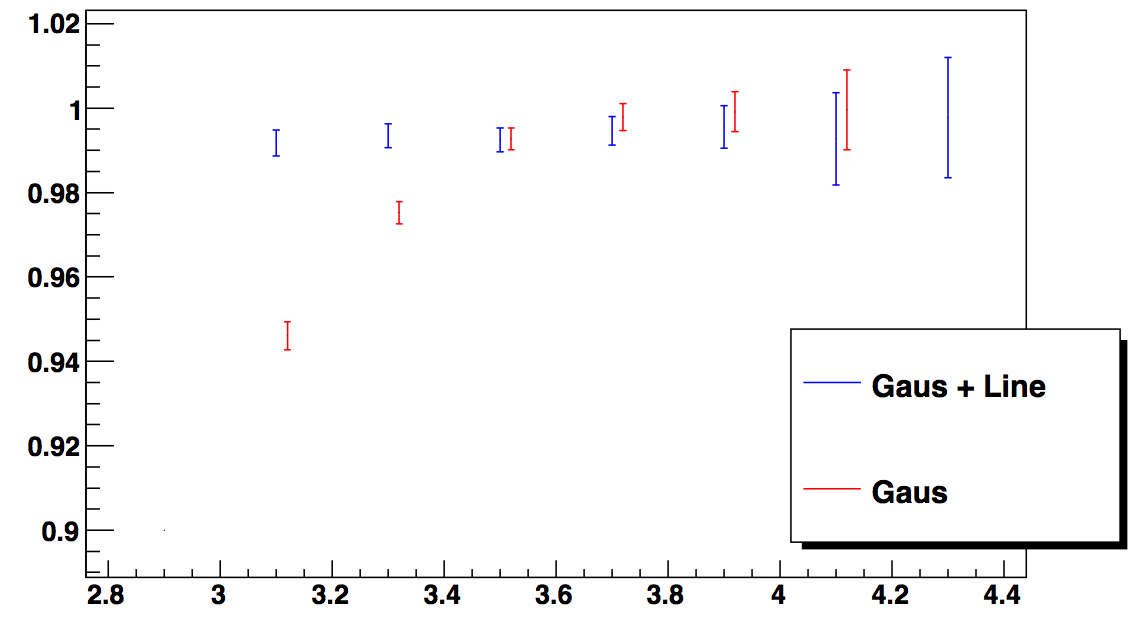
Figure 3 shows the E/p location (y-axis) for different annuli in dR (x-axis/1000), which motivated our dR cut to stay in a flat region:
.png)
After making all of these cuts, we fit E/p to the entire sample of all our electrons. We then add different cuts based on the trigger information to see how that might affect the bias. We looked at four scenarios:
List 2:
- All electrons after stringent cuts
- Electrons from events that were NOT HT/HTTP triggered
- Electrons from events that were only HT/HTTP triggered
- Electrons from HT/HTTP events with trigger turnon tracks (4.5 < p < 6.5 GeV) removed
From these scenarios we chose the largest deviation from E/p = 1.0 as the overall uncertainty on the calibration. This happens to be scenario 3, working out to 1.3%.
Figure 4: E/p for different scenarios
.png)
We also observed a possible crate systematic by fitting E/p for each crate separately.
Figure 5 E/p for each crate:
.png)
According to the chi^2, there is a non statistical fluctuation. To figure out how much that is, we compared the RMS of these points to that when the data is randomly put into 30 partitions. It turns out that all of it is due to that one outlier, crate 12. Since crate 12 contributes 1/15 to each eta ring that it touches, the deviation of this point from the fit causes an uncertainty of 0.9%. This additional uncertainty increases the total uncertainty to 1.6%.
Side Note - Linearity:
After removing HT/HTTP events, we took a look at this plot of p (y-axis) vs E/p (x-axis). By eye, it looks pretty flat, which we verified by splitting into p bins.
Figure 6 p vs E/p
.png)
Figure 7 E/p vs p
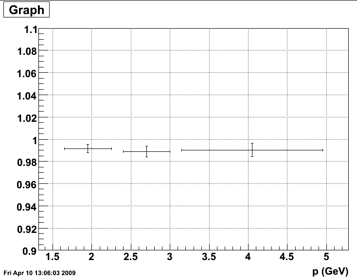
Eta Dependence:
There was some question about whether there was eta dependence. This was investigated and found to be inconsequential: http://drupal.star.bnl.gov/STAR/node/14147/
Figure 8: Divided the sample into 3 separate time periods. Period 1 goes is before run 7110000. Period 2 is between runs 7110000 and 7130000. Period 3 is after run 7130000. The deviations are below 1.6%.
.png)
Figure 9: Agreement between east and west barrel:
.png)
Figure 10: ZDC Rate vs. energy/p
.png)
Figure 11: E/p fits for three different regions in ZDC rate: 0 - 8000, 8000-10000, 10000-20000 Hz.
.png)
Comparison of Electron and MIP Calibrations
This page compares the new tower calibration performed using only electron E/p to the calibration using last year's algorithm. The two calibrations are found to be consistent within 120 MeV in E_T.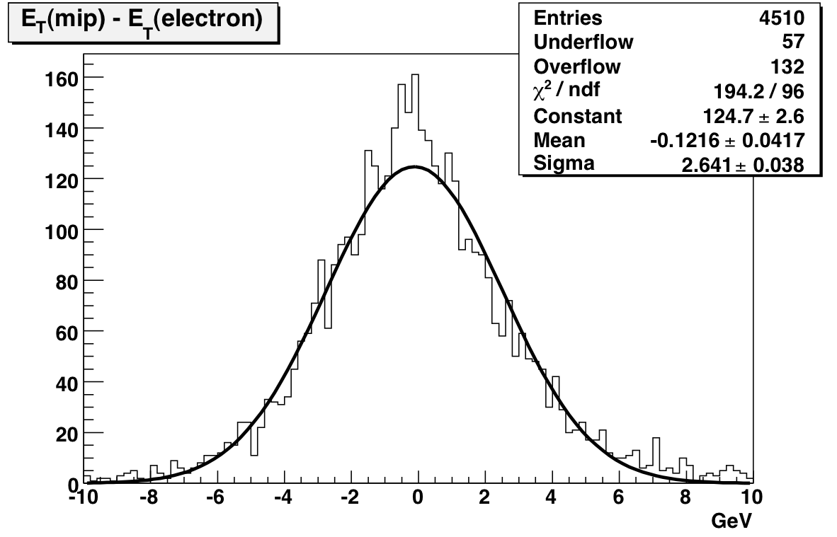
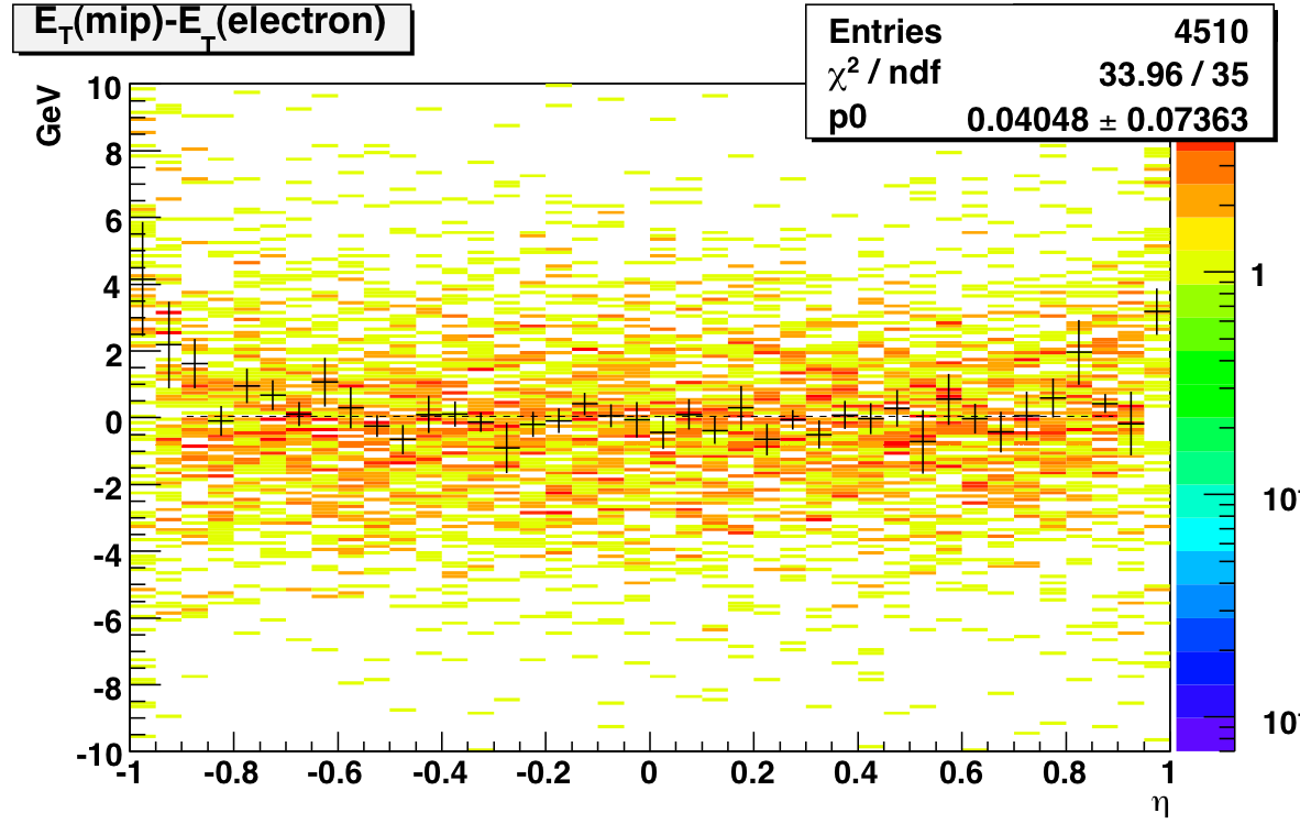
I've also attached the tower-by-tower plots of electron E/p so you can see the results for yourself. I'll write up a more complete description of the calibration algorithm shortly.
Comparison of Online and Offline Calibrations
Introduction:
This page compares the online and first offline calibrations. The online calibration table was generated during data-taking using a single long run processed through fastOffline production and uploaded on March 30th. It uses slopes to set the relative gains in an eta-ring and then normalizes the eta-rings using MIPs. The first offline calibration uses a significant fraction of the produced transverse and late longitudinal runs. It sets the relative gains using MIP peaks and then uses electron E/p to set the absolute scale. It was uploaded on December 7th.Body Counts:
138 additonal towers are masked in this first offline calibration, leaving 4517 good towers. 1 tower (2916) was masked before but is now listed as OK. To be honest, I have no idea why it was masked in the online calib; its slope looks fine to me.Plots:
The electron E/p scaling in the offline calibration increased the gains by an approximately uniform 10 percent (more at the edges). This effect is seen in the following plot of offline E_T - online E_T, integrated over all towers that were good in both calibrations: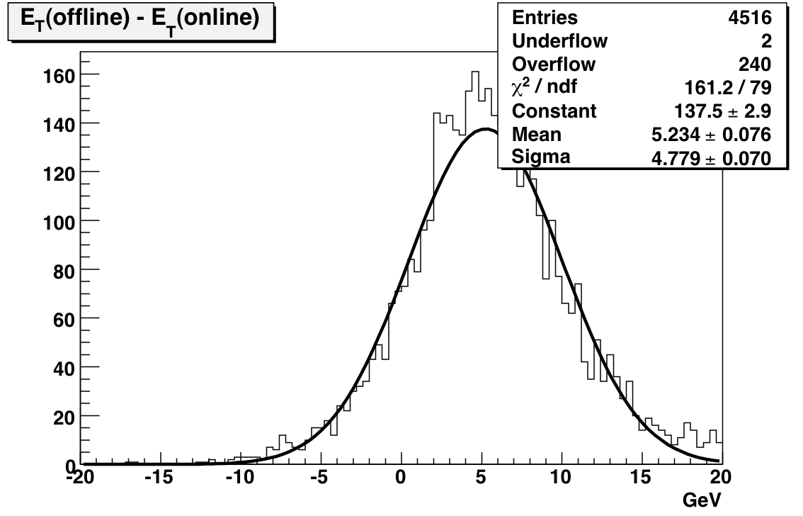
Now, the interesting thing is the relative changes of offline-online for the east side and the west side. If I only plot the location of towers whose gains increased by more than 20% I get
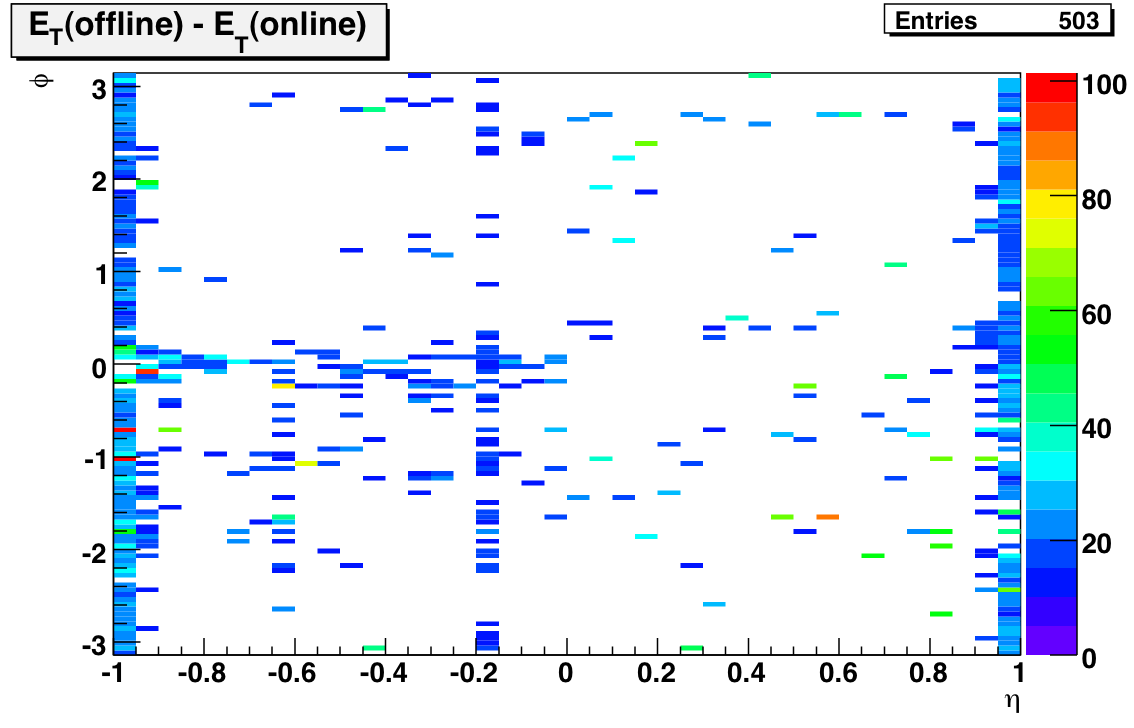
There were only 12 towers whose gains decreased by 20%; all of them were on the west side. Finally here's a plot of the E_T change of the remaining towers:
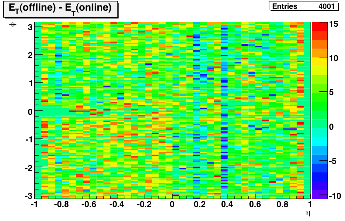
I think the message here is clear: the gains on the east side have increased more than the gains on the west side! It's possible that the use of the online calibration in previous Run 6 jet studies is at least partially responsible for the obsereved east-west jet asymmetry.
To get quantitative about this effect we have to go to 1D. I've attached a PDF of eta-ring by eta-ring histograms like the first one on this page. The first two pages are the east side; the next two are the west side. I've found it easiest to analyze if you set your Reader to view two pages at a time; then you'll be comparing towers with the same absolute value of pseudorapidity when you flip. The conclusion is pretty clear: at midrapidity the difference in offline - online E_T floats around 5 - 8 GeV on the east side, but it's only about 2 - 5 GeV on the west side.
Gain Stability Check
I've updated my codes to do a more systematic investigation of the stability of the gains. Instead of trying to get sufficient tower-by-tower statistics for different time periods, I'm looking at MIP peaks for single runs integrated over all towers. Here's the plot: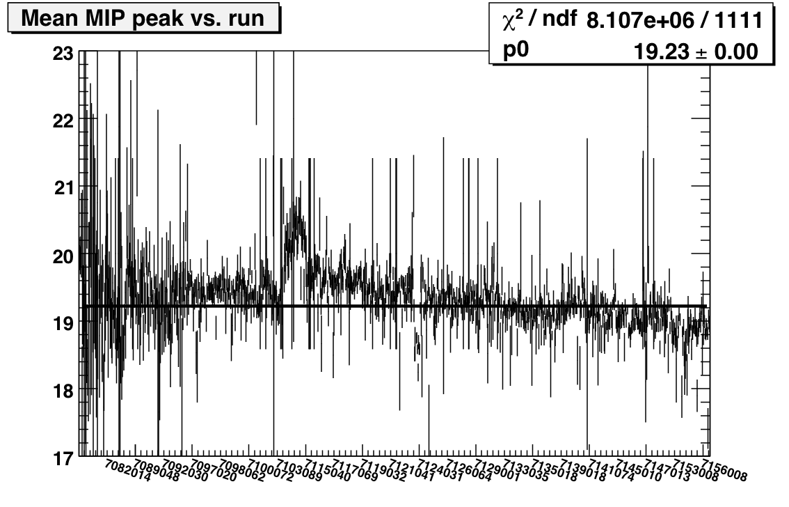
Features of note include the bump covering the first couple of days after the shutdown, the bunch of runs on day 123/4 with very low average peaks, and the general decreasing slope (consistent with towers losing high voltage). I also ran this plot for west and east separately:
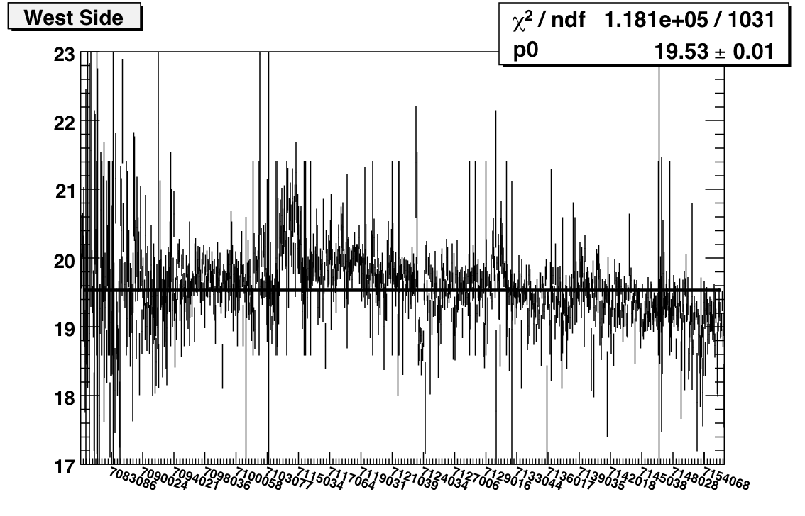
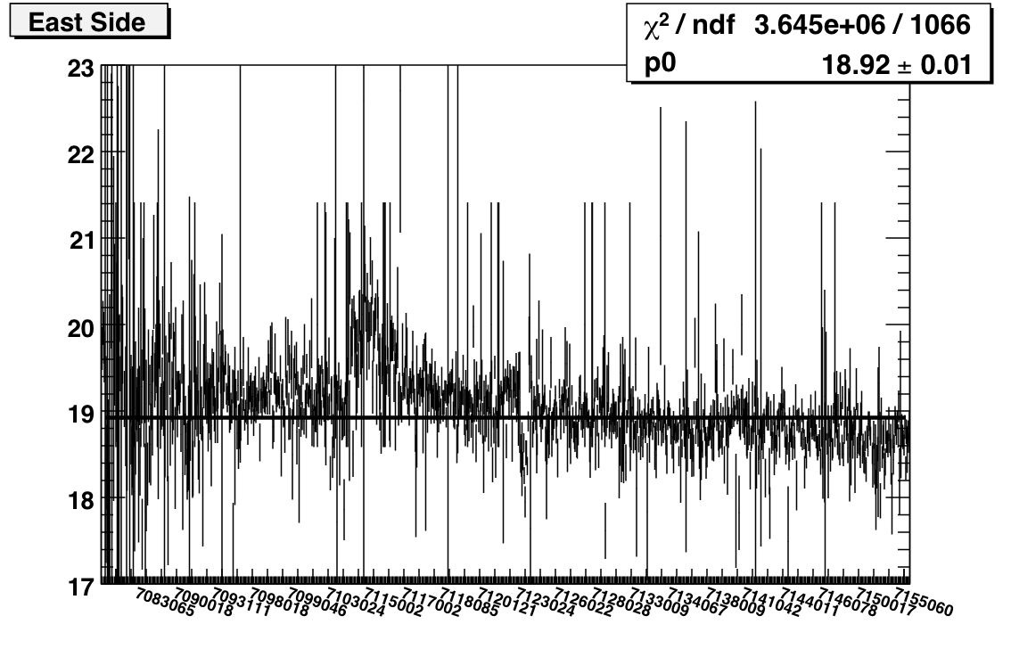
I'm running jobs now to do electron selection instead of MIPs. I think that I can probably still do this as a function of run, but certainly I'll have sufficient stats to plot vs. fill if necessary.
Goal: Compare the tower slopes and MIP peaks from the following three periods to check for stability.
- Day < 104 (97-99)
- 104 < Day < 134 (114-119)
- Day > 134 (134-139)
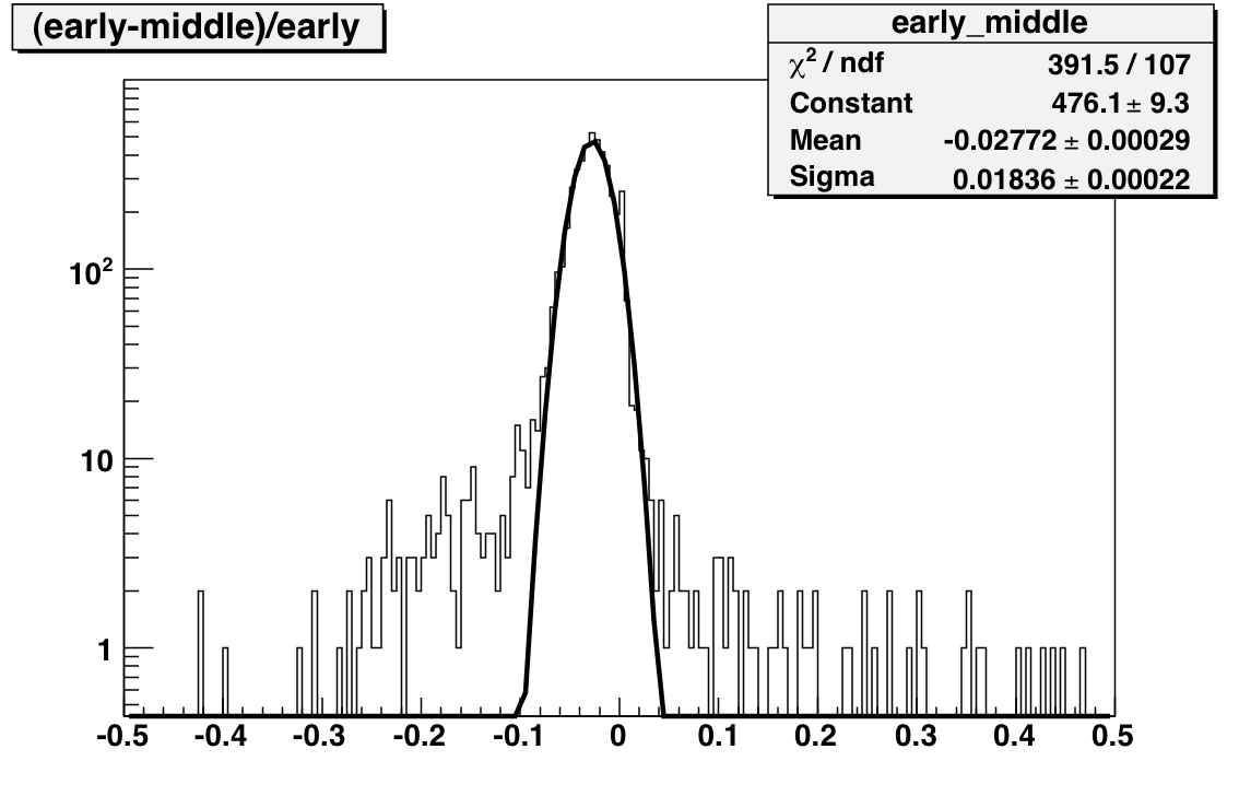
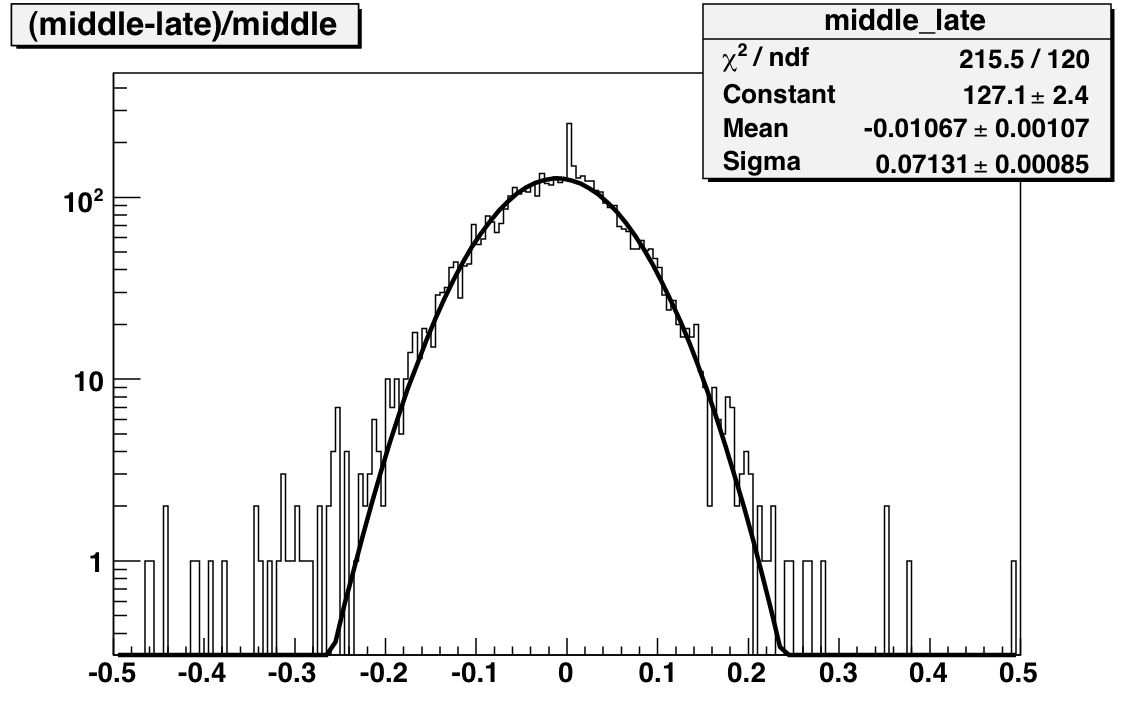
The next set of plots compare gains extracted from MIP peak positions where the MIP peaks are generated using subsets of the Run. Comparing before and after the shutdown yields a mean difference of 110 MeV with a width of 3 GeV. This difference is significantly less than 1 percent. The comparison between middle and late (essentially a comparison between transverse and late longitudinal running) indicates a 1.5 percent drop in the gains with a 2.3 GeV sigma.
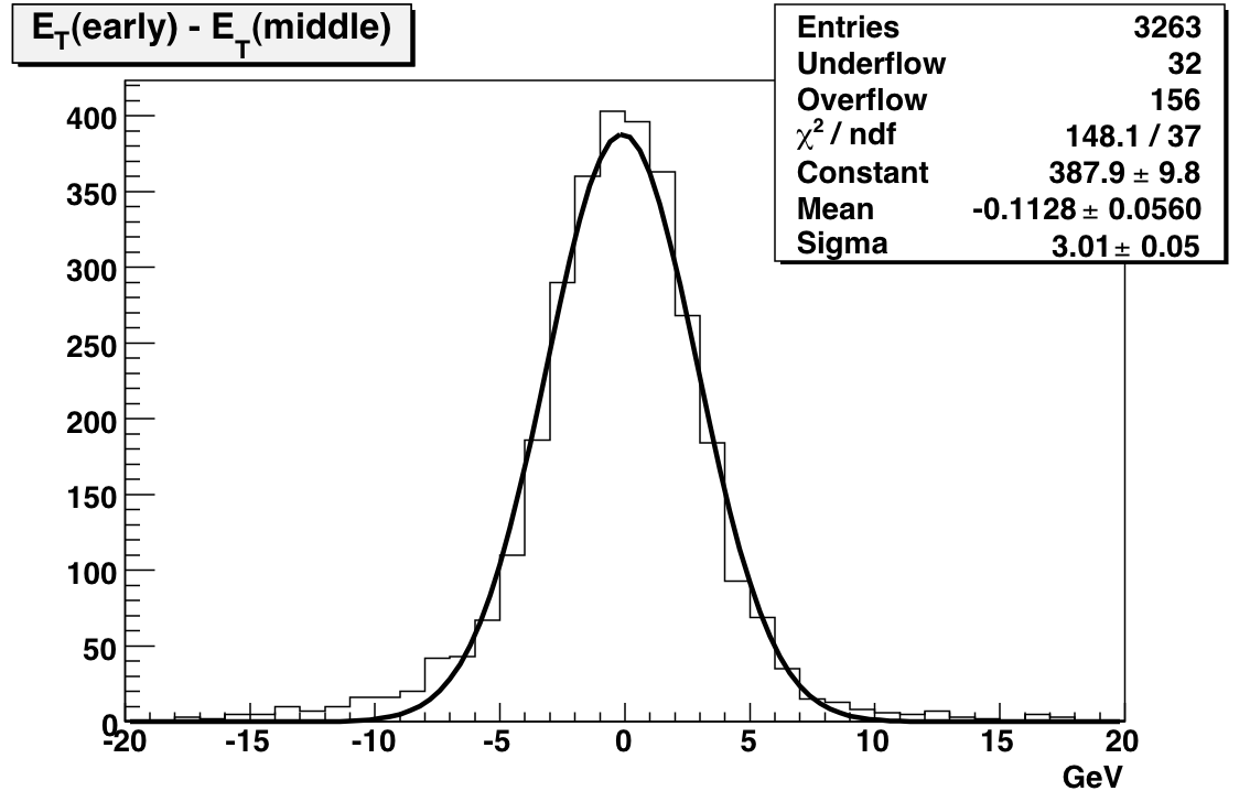
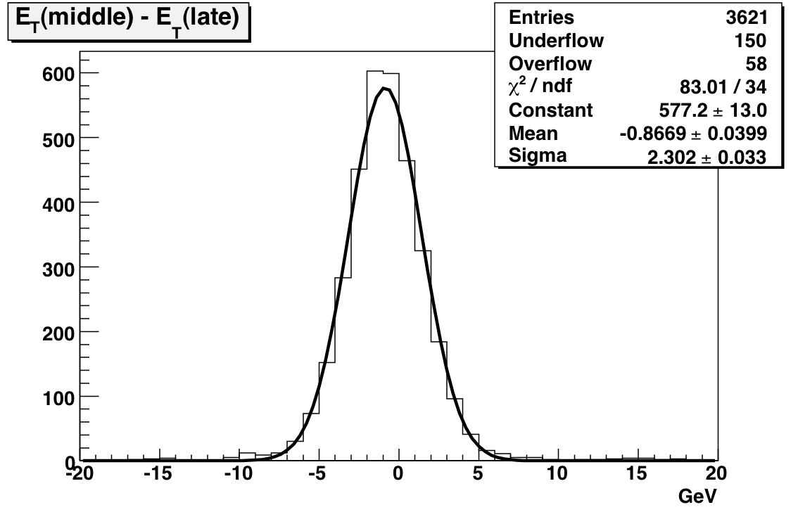
Run 7 BTOW Calibration
Online Work
Steve T's page:http://orion.star.bnl.gov/protected/spin/trent/calibration/calibration.html
First Iteration
March 27, 2007Steve and Oleg took 600k fast events in runs 8086057, 8086058, and 8086060 to calculate the tower slopes. Here's a summary plot of tower slopes vs. eta:
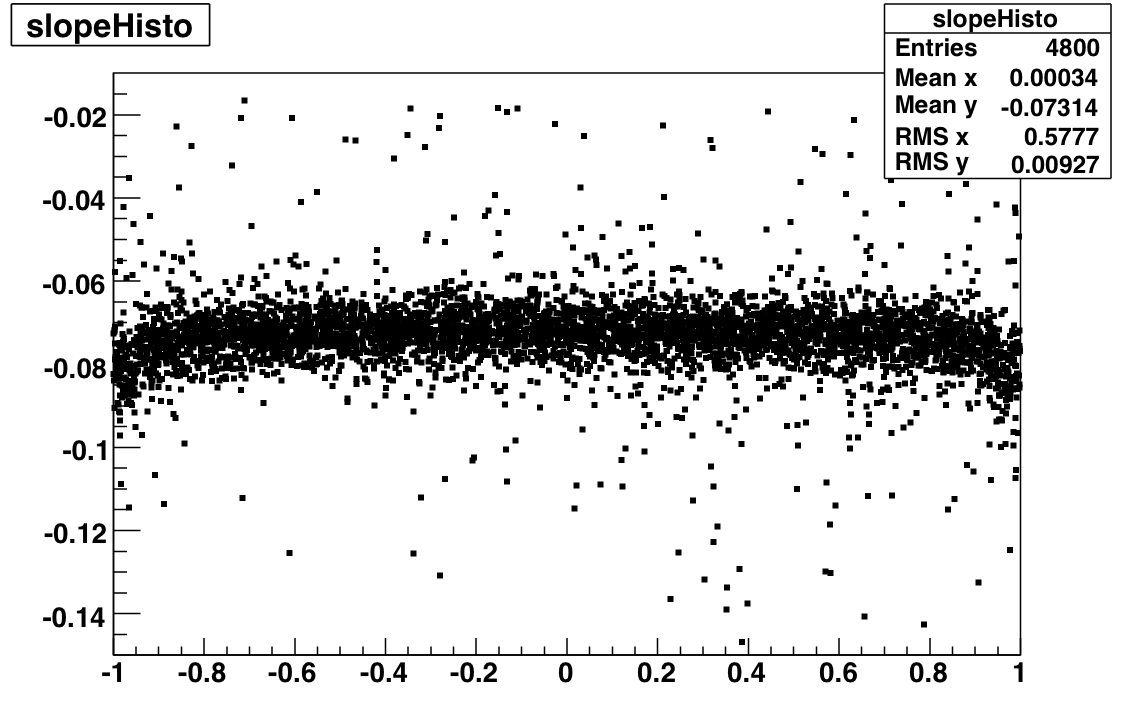
I've attached two list of slopes for each tower at the bottom of the page. The columns are
id -- flag -- slope -- error -- chi2 -- ndf
where the flag is determined by
if(ndf < 30) x //empty, stuck bit
else if(chi2 > 200.) ? //worth a closer look
else if(slope outside 4*RMS) * //probably needs HV adjustment
else blank //channel OK at 4*RMS level
The file slopes_noflags.txt has the same data as the first file, but it omits all the flag information so that it can be read into a macro easily. Flagged channels are also listed in red in the mega-PDF
Second Iteration
Same procedure as First Iteration. Took 600k events in runs 8089017, 8089019, 8089021. This time the processing went smoothly and I was able to analyze ~all the events that were taken. Here's the summary of slopes vs. eta: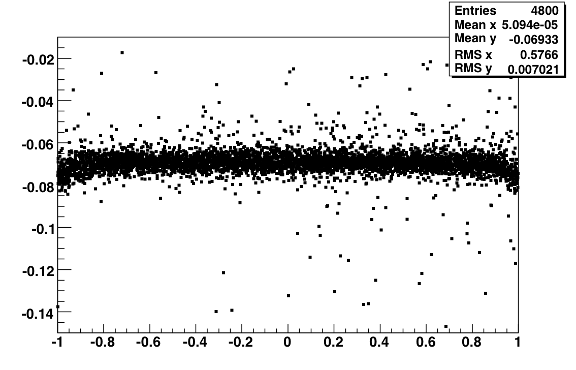
I've attached at the bottom of the page lists of slopes for individual towers. The format is the same as before, although I've adjusted the chi2 cut to 300 because of the additional statistics and I've also adjusted the 4*RMS slope cut to take into account the updated mean and RMS values from the plot above.
Third Iteration
Data gathered from runs 8090021, 8090022, 8090023. The only change I made to the code was to tweak the parameters of the pedestal fit a little bit, since I noticed a couple of towers where it failed.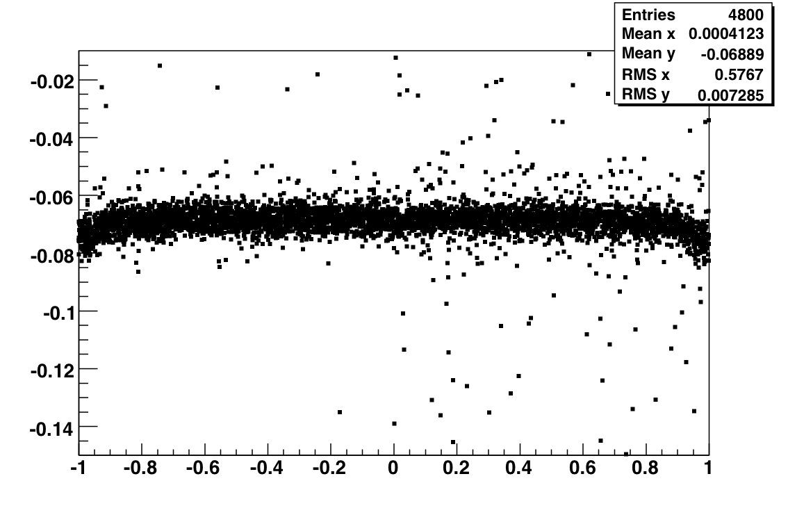
Fourth Iteration
Data gathered from Runs 8091003, 8091005, 8091007. Same analysis codes as in Third Iteration.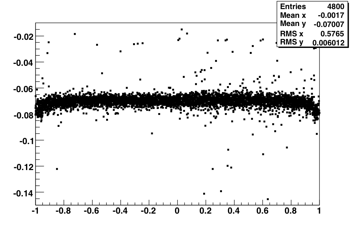
Fifth Iteration
Runs: 8092080, 8092081, 8092083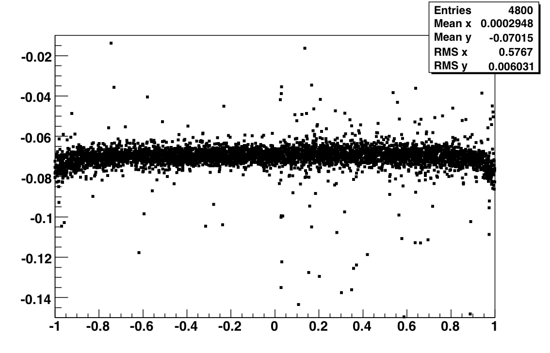
Seventh Iteration
Run 8095073, 600k events.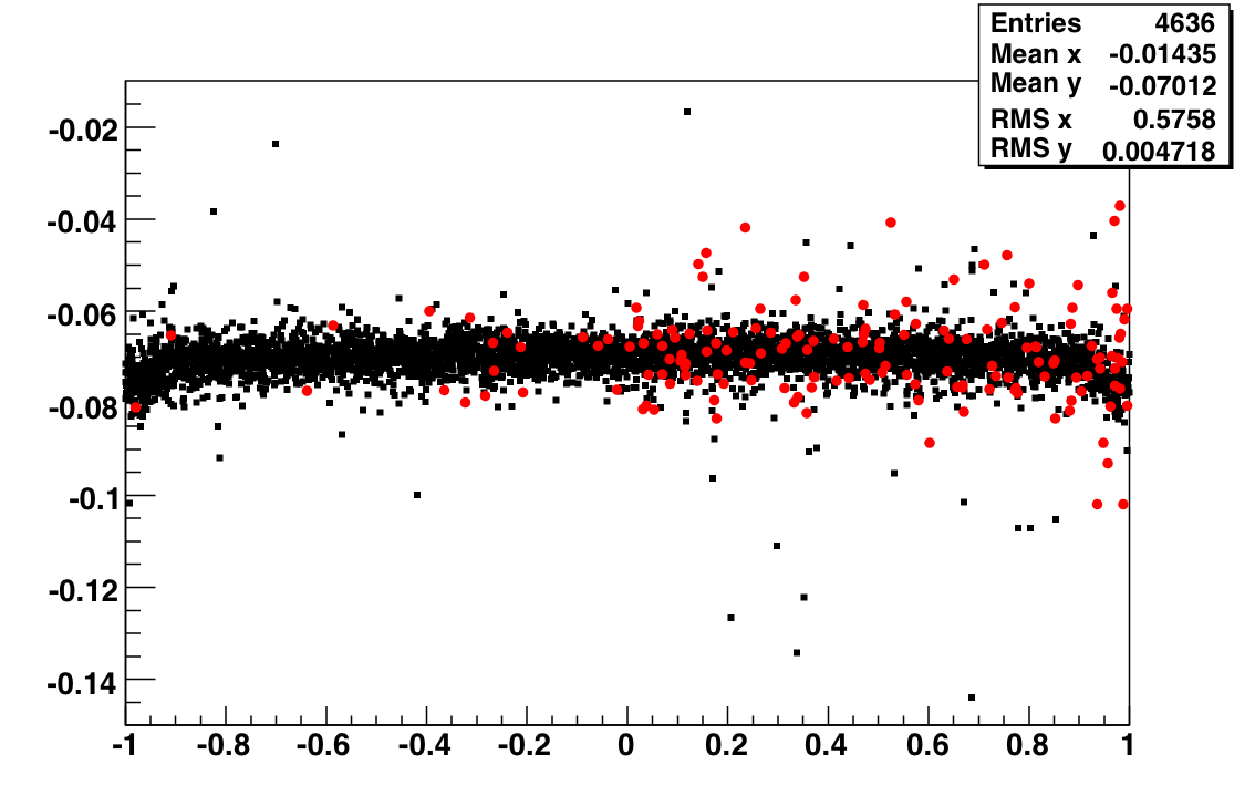
This summary plot highlights swapped towers in red. As Steve pointed out, we weren't adjusting the HV of these tubes correctly in most of the previous iterations.
Run 8 BTOW Calibration (2008)
2008 BTOW calibrations
- BTOW HV used in 2008 are in the file 2008_i2a.csv, this file will contain a few towers
(<50)which might have been set to zero at a later date
01 statistical analysis of 2008 HV
Goal: study eta dependence of 2008 BTOW HV
Fig 1 Eta-phi distribution of HV

Formulas used to map tower ID in to eta-phi location
    int id0=id-1;
    int iwe=0; // West/East switch
    if(id>2400) iwe=1;
    int id0=id0%2400;
    int iphi=id0/20;
    int ieta=id0%20;
    if(iwe==0) ieta=ieta+20;
    else ieta=19-ieta;
Fig 2 Batch 1, Eta-phi distribution of HV

eta=0.05  mean HV=821 +/- 5  sigHV=60
eta=0.15  mean HV=820 +/- 5  sigHV=60
eta=0.25  mean HV=815 +/- 5  sigHV=62
eta=0.35  mean HV=811 +/- 5  sigHV=66
eta=0.45  mean HV=817 +/- 5  sigHV=66
eta=0.55  mean HV=820 +/- 5  sigHV=57
eta=0.65  mean HV=820 +/- 5  sigHV=59
eta=0.75  mean HV=806 +/- 5  sigHV=62
eta=0.85  mean HV=807 +/- 5  sigHV=58
eta=0.95  mean HV=829 +/- 5  sigHV=65
Fig 3 Batch 2, Eta-phi distribution of HV

eta=0.05  mean HV=759 +/- 6  sigHV=56
eta=0.15  mean HV=760 +/- 7  sigHV=62
eta=0.25  mean HV=756 +/- 6  sigHV=53
eta=0.35  mean HV=763 +/- 6  sigHV=55
eta=0.45  mean HV=756 +/- 7  sigHV=58
eta=0.55  mean HV=760 +/- 6  sigHV=54
eta=0.65  mean HV=743 +/- 6  sigHV=52
eta=0.75  mean HV=754 +/- 6  sigHV=54
eta=0.85  mean HV=754 +/- 7  sigHV=64
eta=0.95  mean HV=769 +/- 7  sigHV=59
Fig 4 Batch 3, Eta-phi distribution of HV

eta=-0.95  mean HV=730 +/- 4  sigHV=57
eta=-0.85  mean HV=723 +/- 4  sigHV=57
eta=-0.75  mean HV=727 +/- 4  sigHV=59
eta=-0.65  mean HV=718 +/- 4  sigHV=58
eta=-0.55  mean HV=723 +/- 4  sigHV=58
eta=-0.45  mean HV=720 +/- 4  sigHV=56
eta=-0.35  mean HV=727 +/- 4  sigHV=54
eta=-0.25  mean HV=724 +/- 4  sigHV=60
eta=-0.15  mean HV=735 +/- 4  sigHV=59
eta=-0.05  mean HV=729 +/- 4  sigHV=60
02 BTOW swaps ver=1.3
Example of MIP peak for BTOW towers pointed by TPC MIP track:  Spectra for 4800 towers (raw & MIP) are in attachment 1.
Method of finding MIP signal in towers:

Table 1
BTOW swaps, very likely, ver 1.3, based on 2008 pp data, fmsslow-production
 266 --> 286 , 267 --> 287 , 286 --> 266 , 287 --> 267 , 389 --> 412 ,
 390 --> 411 , 391 --> 410 , 392 --> 409 , 409 --> 392 , 410 --> 391 ,
 411 --> 390 , 412 --> 389 , 633 --> 653 , 653 --> 633 , 837 --> 857 ,
 857 --> 837 ,1026 -->1046 ,1028 -->1048 ,1046 -->1026 ,1048 -->1028 ,
1080 -->1100 ,1100 -->1080 ,1141 -->1153 ,1142 -->1154 ,1143 -->1155 ,
1144 -->1156 ,1153 -->1141 ,1154 -->1142 ,1155 -->1143 ,1156 -->1144 ,
1161 -->1173 ,1162 -->1174 ,1163 -->1175 ,1164 -->1176 ,1173 -->1161 ,
1174 -->1162 ,1175 -->1163 ,1176 -->1164 ,1753 -->1773 ,1773 -->1753 ,
2077 -->2097 ,2097 -->2077 ,3678 -->3679 ,3679 -->3678 ,3745 -->3746 ,
3746 -->3745 ,4014 -->4054 ,4015 -->4055 ,4016 -->4056 ,4017 -->4057 ,
4054 -->4014 ,4055 -->4015 ,4056 -->4016 ,4057 -->4017 ,4549 -->4569 ,
4569 -->4549 ,
Details for all swaps are shown in attached 2.
Other problems found during analysis, not corrected for, FYI

03 MIP peak analysis (TPC tracks, 2008 pp data)
I examined runs from 2008 pp (list attached below) to create calibration trees (using StRoot/StEmcPool/StEmcOfflineCalibrationMaker). The code loops over the primary tracks in the event and selects the global track associated with it, if available. If the track can be associated to a tower and has outermomentum > 1 GeV, it is saved.
I then loop over those tracks and choose ones that fall within a certain criteria:
- p > 1
- adc - ped > 1.5 * ped_rms
- tower_entrance_id = tower_exit_id
- only a single track points to the tower
- neighoring towers have small amounts of energy
We can sum over all runs to produce MIP spectrum in 4445 towers. Of those, 4350 pass current QA requirements. An example MIP spectrum with fit is shown below. All MIP peaks can be seen in the attached PDF. It's important to note that the uncertainty on the MIP peak location with these statistics is on average 5%. This number is a lower limit on the calibration coefficient uncertainty that can only be improved with statistics.
Fig 1. Typical MIP peak. Plots like this for all 4800 towers are in attachment 1.
The following plot shows MIP peak location in ADCs (in eta, phi space) of all of towers where such a peak could be found.
Fig 2. MIP Peak (Z-axis) for all towers
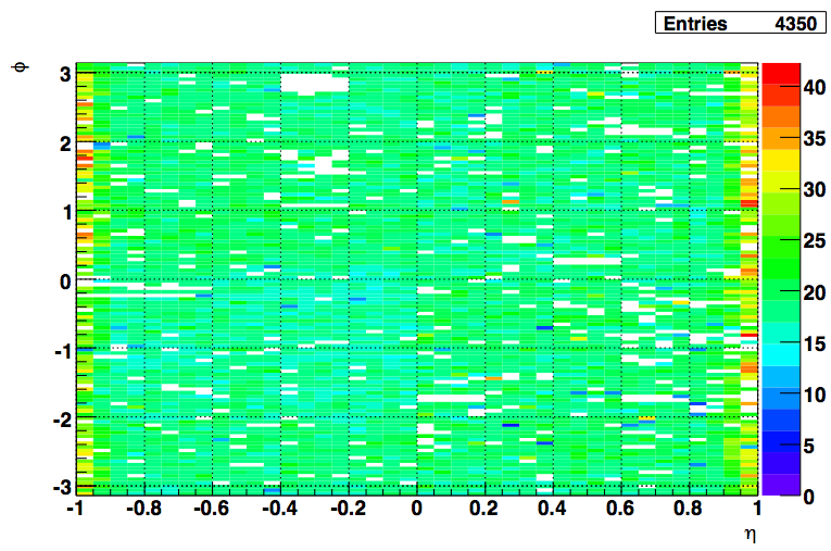
This plot shows the status codes of the towers. White are the towers that had 0 entries in their histograms. Red are the good towers (pushed them off scale to see the rest of the entries). Towers in the outermost eta bin received different treatment. The fit range was between [6,100] for those towers (vs [6,50] for the rest). The cuts applied for QA were slightly loosened. The rest of the codes follow this scheme:
- bit 1: entries in histogram > 0
- bit 2: sigma of fit below threshold (15,20)
- bit 4: mean of fit above 5 ADCs
- bit 8: difference of fit mean and MPV in fit range below threshold (5,10)
Fig 3. status of towers
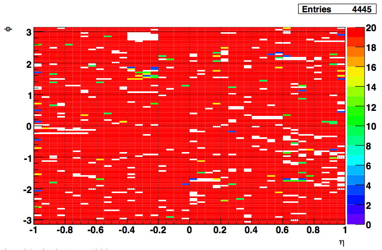
Spectra of towers rejected by rudimentary automatic QA were manually inspected and 91 were found to contain reasonable MIP peak and have bin re-qualified as good. PLots for those towers are in attachment 2.
04 relative tower gains based on MIPs (gain correction 1)
Determination of relative gains BTOW gains based on MIP peak for the purpose of balancing HV for 2009 run
Procedure:
- use fitted 03 MIP peak analysis (TPC tracks, 2008 pp data)
- find average MIP value for 40 eta bins
- West barrel: preserve absolute average MIP peak position in the , compute gain correction to equalize all towers at given eta to the average for this eta
- East barrel: enforce absolute average MIP peak to agree with the West barrel, correct relative gains in the similar way.
In this stage of calibration process 4430 towers with well visible MIP peak were use. The remaining 370 towers will be called 'blank towers' . There are many reasons MIP peak doe snot show up e.g. dead hardware. ~60 of the 'blank towers' are 02 BTOW swaps ver=1.3- as identified earlier and not corrected in this analysis.
Fig 1. Left: MIP peak (Z-axis) was found for 4430 towers shown in color. White means no peak was found - those are "blank towers". Right: eta-phi distribution of blank towers. On both plots East (West) barrel is show on etaBins [1-20], (21,40).

The (iEta, iPhi ) coordinates were computed based on softID as follows:
   int jeta= 1+(id-1)%20; // range [1-20]
   int jphi= 1+(id-1)/20; // range [1-240]
   if(jphi<=120) { // West barrel
      keta=jeta+20; kphi=jphi;
   } else { // East barrel
      keta=-jeta+21; kphi=jphi-120;
   }
Fig 2. Average MIP position as function of eta bin. West-barrel gains are higher even of average.

Gain corrections (GC1) were computed as
GC1(iEta,iPhi)= MIP(iEta,iPhi) / avrMip(iEta)
For the East-barrel we used values of avrMip(iEta)from symmetric eta-bins from the West barrel.
If computed correction was between [0.95,1.05] or if towers was "blank" GC1=1.00 was used.
Fig 3. Left distribution of gain corrections GC1(iEta). Right: value of GC1(iEta,iPhi).

Attached spreadsheet contains computed GC1(softID) in column 'D' together with MIP peak parameters (columns H-P) for all 4800 towers. Below is just first 14 towers.

Used .C macro is attached as well.
05 Absolute Calibration from Electrons
We use the MIP ADC location calculated in part 03 to get a preliminary measure of the energy scale for each tower.
The following formula from SN436 provides the calibration coefficient:
C = 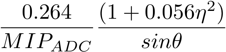
where E = C * (ADC - ped).
For the electron sample I select tracks with:
- 1.5 < p < 6.0 (GeV)
- dR < 0.0125 (from center of face of tower in eta/phi space)
- adc - ped > 2.5 * ped_rms in tower
- nHits > 10
- nSigmaElectron > -1
Here is one of the E/p distributions. Note the error on the mean is about 2%, which is about average.
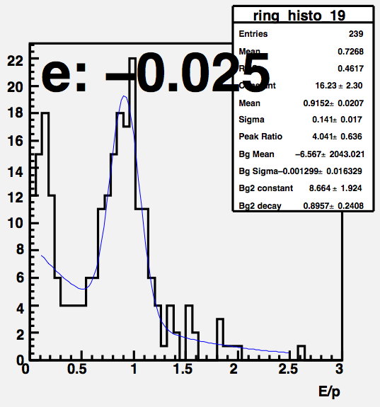
For each electron we calculate E/p and sum over eta rings. Here is the peak of E/p for each eta bin. The error bars show the error on the mean value, and the shaded bar is the sigma. I fit over the range [-0.9,0.0] and [0.0,0.9] separately. The fit for the east reports the mean is 0.9299 +/- 0.0037. For the west, I get 0.9417 +/- 0.0035.
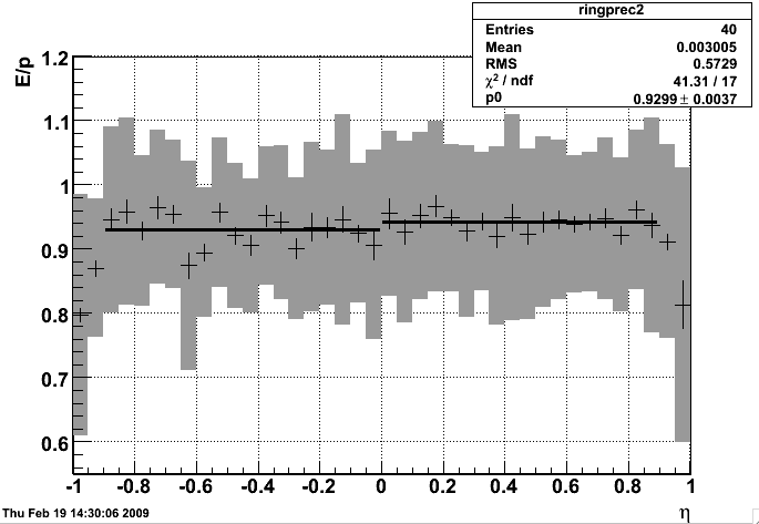
The location of the E/p peak tells us the correction that needs to be applied to the calibration coefficients of towers in each eta ring to get the correct absolute energy.
Reference plot (electron showers):
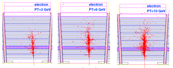
06 Calculating 2009 HV from Electron Calibrations
The ideal gain for each tower satisfies the following relation, where E_T = 60 GeV when ADC is max scale (~4095 - ped):
(1)
We want to calculate the total energy deposited in a tower, which is the following in the ideal case:
(2)
In reality, we calculate the calibration according to the following formula:
(3)
where there is an electron correction for each eta ring, and the MIP location is determined for all towers.
Thus, to have ideal gains, we want the following relation to hold
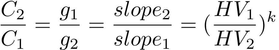 (4)
(4)
To make this relation true, we need to adjust the high voltage for each tower according to the following relation:
(5)
We can check the changes using slopes.
07 BTOW absolute gains 'ab initio'
Summary of intended BTOW HV change, February 24, 2009
Conclusion:
We will NOT change average gain of West BTOW for eta bins[1,18]. For all other eta bins we will aim at the average West Btow marked as red dashed line.

Full presentation is in attachment 1.
Detailed E/P spectra for 40 eta bins are in attachment 2 & 3.
08 Completed Calibration and Uncertainty
The 2008 Calibraton has been uploaded into the database. I was able to find calibration coefficients for 4420 towers. Of the remaining towers, 353 were MIPless and 27 had spectrums that I could not recover by hand.
This year, differently from previous years, known sources of bias are removed. If an event had a nonHT trigger, the tracks from that event were used for the calibration (even if it had an HT trigger). Most of the triggers were fms slow triggered events. Each eta ring was calibrated separately, and then a correction for each crate was applied. After these corrections, I once again made the cuts on the electrons more stringent. No deviation from E/p =1 was found. With the biases eliminated, we now quote a systematic variance instead of a systematic bias as the uncertainty on the calibration.
The source of this uncertainty are the uncertainties on various fits used for each calibration, namely the MIP peak for each tower, the absolute calibration for each eta ring, and the correction for each crate. These uncertainties are highly correlated. I have completed this calibration by recalculating the calibration table 3,000 times varying the MIP peaks, the eta ring corrrections and the crate corrections each time. Using this method, I was able to determine the correlated uncertainty for each calibrated tower. This uncertainty is, on average, 5%.
This uncertainty is different than the systematic bias quoted for 2005 and 2006. It is a true variance on the calibration. To use this uncertainty, analyzers should recalculated their analysis using test tables generated for this purpose. The variance in the results of these multiple analyses will give a direct measure of the uncertainty due to the calibration scale uncertainty. These tables will be uploaded to the database with the names "sysNN". They should be used before clustering, jet finding, etc.
Run 9 BTOW Calibration
Parent page for BTOW 2009 Calibrations
01 BTOW HV Mapping
We started at the beginning of the run to verify the mapping between the HV cell Id and the softId it corresponds to. To begin, Stephen took 7 runs with all towers at 300V below nominal voltage except for softId % 7 == i, where i was different for each run. Here are the runs that were used:
| softId%7 | Run Number | Events |
| 1 | 10062047 | 31k |
| 2 | 10062048 | 50k |
| 3 | 10062049 | 50k |
| 4 | 10062050 | 50k |
| 5 | 10062051 | 50k |
| 6 | 10062060 | 100k |
| 0 | 10062061 | 100k |
We used the attached file 2009_i0.txt (converted to csv) as the HV file. This file uses the voltages from 2008 and has swaps from 2007 applied. Swaps indentified were not applied and will be used to verify the map check.
File 2009_i0c.txt contains some swaps identified by the analysis of these runs.
File 2009_i1c.txt contains adjusted HV settings based on the electron/mip analysis with same mapping as 2009_i0c.txt.
Final 2009 BTOW HV set on March 14=day=73, Run 10073039 , HV file: 2009_i2d.csv
02 Comparing 2007, 2008 and 2009 BTOW Slopes
We have taken two sets of 1M pp events at sqrt(s)=500 GeV. For future reference, the statistical error on the slopes is typically in the range of 3.7%. I give a plot of the relative errors in the 5th attachment.
plus we have
Comparing the overall uniformity of the gain settings, I give the distribution of slopes divided by the average over the region |ETA|<0.8 for 2007, 2008 and 2009 (First three attachments)
I find that there is little difference in the overall uniformity of the slopes distribution over the detector...about +/-5%. I also give a plot showing the average slopes in each eta ring for the three different voltage settings in each year 2007. 2008 and 2009. (4th attachment) As you can see, the outer eta rings were overcorrected in 2008. They are now back to nearly the same positions as in 2007.
_________________________________________________________________
Here is my measurement of 'kappa' from 2007 data. I get from 7-8, depending on how stringent the cuts are. I think this method of determining kappa is dependent on the ADC fitting range. In theory, we should approach kappa~10.6 as we converge to smaller voltage shifts.
So which ones should we adjust? Here is a fit of the slope distribution to a gaussian.
As we can see, the distribution has an excess of towers with slopes >+/-20% from the average. I checked that these problem towers are not overwhelmingly swapped towers (15/114 outliers are swapped towers; 191/4712 are swapped towers). Here is an eta:phi distribution (phi is SoftId/20%120, NOT angle!). The graph on the left gives ALL outliers, the graph on the right gives outliers with high slopes only (low voltage). There are slightly more than expected in the eta~1 ring, indicating that the voltages for this ring are set to accept few particles than the center of the barrel.
______________________________________________________________________
So Oleg Tsai and I propose to change only those outliers which satisfy the criteria:
|slope/ave_slope - 1|>0.2 && |eta|<0.8. (Total of 84 tubes)
We then looked one-by-one thru the spectra for all these tubes (Run 10066010) and found 12 tubes (not 13 as I stated in my email) with strange spectra:
Bad ADC Channels: Mask HV to Zero
We then calculated the proposed changes to the 2009_i1c.csv HV using the exponent kappa=5. Direct inspection of the spectra made us feel as though the predicted voltage changes were too large, so we recomputed them using kappa=10.48. We give a file containing a summary of these changes:
Proposed HV Changes (SoftId SwappedID Slope(i1c) Ave Slope Voltage(i1c) New Voltage
(We have identified 3 extra tubes with |eta|>0.8 which were masked out of the HT trigger to make it cleaner....we propose to add them to list to make a total of 87-7 = 80 HV changes.)
PS. We would also like to add SoftId-3017 HV800 -> 650. This make 81 HV changes.
_____________________________________________________________________
A word about stability of the PMT High Voltage and these measurements. I compared several pairs of measurements in 2007 taken days apart. Here is an intercomparison of 3 measurements (4,5 and 7) taken in 2007. The slopes have a statistical accuracy of 1.4%, so the distribution of the ratio of the two measurements should have a width of sqrt(2)*1.4 = 2% The comparison of the two measurements is just what we expect from the statistical accuracy of the slope measurements.
Comparing the two recent measurements in 2009, we have a set of about 600 tubes with a very small voltage change. The slopes were measured with an accuracy of 3.7%, so the width of the slope ratio distribution should be sqrt(2)*3.7% =5.2%. Again, this is exactly what we see. I do not find any evidence that (a large percentage of) the voltages are unstable!
___________________________________________________________________
03 study of 2009 slopes (jan)
Purpose of this study is to evaluate how successful was our firts attempt to compute new 2009 HV for BTOW.
Short answer: we undershoot by a factor of 2 in HV power- see fig 4 left.
Input runs: 10066160 (new HV) and 10066163 (old HV)
Fig 1. Pedestal distribution and difference of peds between runs - perfect. Peds are stable, we can use the same slope fit range (ped+20,ped+60) blindly for old & new HV.

Fig 2. Chosen HV change and resulting ratio of slopes - we got the sign of HV change correctly!

Fig 3. Stability test. Plots as in fig 2, but for a subset of towers we change HV almost nothing (below 2V) but yield was large. One would hope slope stay put. They don't. This means either slopes are not as reliable as we think or HV is not as stable as we think.

Fig 4. Computed 'kappa' : sl2/sl1=g1/g2=V1/V2^kappa for towers with good stats and HV change of at least 10 Volts, i.e. the relative HV change is more than 1%. Right plot shows kappa as function of eta - no trend but the distribution is getting wider - no clue why?

Fig 5. Computed 'kappa' as on fig 4. Now negative, none physical values of kappa are allowed.

04 Spectra from Problem PMT Channels
We set the HV = 800 Volts for all channels which have been masked out, repaired, or otherwise had problems in 2008. I have examined the spectra for these channels and give pdfs with each of these spectra:
drupal.star.bnl.gov/STAR/system/files/2009_800_1_12.pdf
drupal.star.bnl.gov/STAR/system/files/2009_800_13_24.pdf
drupal.star.bnl.gov/STAR/system/files/2009_800_25_36.pdf
drupal.star.bnl.gov/STAR/system/files/2009_800_37_48.pdf
drupal.star.bnl.gov/STAR/system/files/2009_800_49_60.pdf
drupal.star.bnl.gov/STAR/system/files/2009_800_61_72.pdf
drupal.star.bnl.gov/STAR/system/files/2009_800_72_78.pdf
I identify 37 tubes which are dead, 39 tubes which can be adjusted, and 1 with a bit problem. We should pay careful attention to these tubes in the next iteration.
05 Summary of HV Adjustment Procedure
Summary of process used to change the HV for 2009 in BTOW:HV Files: Version indicates interation/mapping (numeral/letter)
1) 2009_i0.csv HV/Mapping as set in 2008. Calibration determined from 2008 data electrons/MIPS.
http://drupal.star.bnl.gov/STAR/subsys/bemc/calibrations/run-8-btow-calibration-2008/05-absolute-calibration-electrons
2) 2009_i0d.csv Map of SoftId/CellId determined by taking 6 data sets with all voltages set to 300 V, except for SoftId%6=0,1,2,3,4,5,6, successively. (link to Joe's pages)
http://drupal.star.bnl.gov/STAR/subsys/bemc/calibrations/run-8-btow-calibration-2008/08-btow-hv-mapping
drupal.star.bnl.gov/STAR/blog-entry/seelej/2009/mar/10/run9-btow-hv-mapping-analysis-summary
drupal.star.bnl.gov/STAR/blog-entry/seelej/2009/mar/05/run9-btow-hv-mapping-analysis
drupal.star.bnl.gov/STAR/blog-entry/seelej/2009/mar/08/run9-btow-hv-mapping-analysis-part-2
3) 2009_i1d.csv HV change determined from 2008 data electrons/MIPS (g1/g2)=(V2/V1)**k, with k=10.6 (determined from LED data).
http://drupal.star.bnl.gov/STAR/subsys/bemc/calibrations/run-8-btow-calibration-2008/06-calculating-2009-hv-electron-calibrations
4) 2009_i2d.csv Slopes measured for all channels. Outliers defined as |slope/<slope> -1|>0.2 (deviation of channel slope from average slope over barrel >20%:Approx 114 channels. Outliers corrected according to (s1/s2)=(V1/V2)**k as above. Hot towers HV reduced by hand. (Approx 10 towers)
http://drupal.star.bnl.gov/STAR/subsys/bemc/calibrations/run-9-btow-calibration-page/02-comparing-2007-2008-and-2009-btow-slopes
06 comparison of BTOW status bits L2ped vs. L2W , pp 500 (jan)
Comparison of BTOW status tables generated based on minB spectra collected by L2ped ( conventional method) vs. analysis of BHT3 triggered , inclusive spectra.
- Details of the method are given at BTOW status table algo, pp 500 run, in short status is decided based on ADC integral [20,80] above pedestal.
- the only adjusted param is 'threshold' for Int[20,80]/Neve*1000. Two used values are 1.0 and 0.2.
- For comparison I selected 2 fills: F10434 (day 85, ~all worked) and F10525 (day99, 2 small 'holes' in BTOW) - both have sufficient stats in minB spectra to produce conventional status table.
- Matt suggested the following assignment of BTOW status bits (value of 2N is given)
- good -->stat=1
- bad, below thres=0.2 --> stat=2+16 (similar to minB cold tower)
- bad, below thres=1.0 --> stat=512 (new bit, stringent cut for dead towers for W analysis)
- stuck low bits --> stat=8 (not fatal for high-energy response expected for Ws)
- broken FEE (the big hole) in some fills, soft ID [581-660] --> stat=0
Fig 1. Fill F10343 thres=1.0 (red line)

There are 108 towers below the red line, tagged as bad. Comparison to minB-based tower QA which tagged 100 towers. There are 4 combinations for tagging bad towers with 2 different algos. Table 1 shows break down, checking every tower. Attachments a, b show bad & good spectra.
|
|
Conclusion 1: some the additional 8 towers tagged as bad based on BHT3 spectra are either very low HV towers, or optical fiber is partially broken. If those towers are kept for W analysis any ADC recorded by them would yield huge energy. I'd like to exclude them from W analysis anyhow.
To preserve similarity to minB-based BTOW status code Matt agreed we tag as bad-for-everybody all towers rejected by BHT3 status code using lower threshold of 0.2. Towers between BHT3 QA-thresholds [0.2,1.0] will be tagged with new bit in the offline DB and I'll reject them from W-analysis if looking for W-signal but not necessary if calculating the away side ET for vetoing of away side jet.
|
|
Spectra are in attachment c). Majority of towers for which this 2 methods do not agree have softID ~500 - where this 2 holes reside (see 3rd page in PDF)
Tower 220 has stuck lower bits, needs special treatment - I'll add detection (and Rebin()) for such cases.
Automated generation of BTOW status tables for fills listed in Table 3 has been done, attachment d) shows summary of all towers and examples of bad towers for all those fills.
 Table 3
     1  # F10398w  nBadTw=112 totEve=12194
     2  # F10399w  nBadTw=111 totEve=22226
     3  # F10403w  nBadTw=136 totEve=3380
     4  # F10404w  nBadTw=115 totEve=9762
     5  # F10407w  nBadTw=116 totEve=7353
     6  # F10412w  nBadTw=112 totEve=27518
     7  # F10415w  nBadTw=185 totEve=19581
     8  # F10434w  nBadTw=108 totEve=15854
     9  # F10439w  nBadTw=188 totEve=21358
    10  # F10448w  nBadTw=190 totEve=18809
    11  # F10449w  nBadTw=192 totEve=18048
    12  # F10450w  nBadTw=115 totEve=14129
    13  # F10454w  nBadTw=121 totEve=6804
    14  # F10455w  nBadTw=113 totEve=16971
    15  # F10463w  nBadTw=114 totEve=12214
    16  # F10465w  nBadTw=112 totEve=8825
    17  # F10471w  nBadTw=193 totEve=21003
    18  # F10476w  nBadTw=194 totEve=9067
    19  # F10482w  nBadTw=114 totEve=39315
    20  # F10486w  nBadTw=191 totEve=37155
    21  # F10490w  nBadTw=154 totEve=31083
    22  # F10494w  nBadTw=149 totEve=40130
    23  # F10505w  nBadTw=146 totEve=37358
    24  # F10507w  nBadTw=147 totEve=15814
    25  # F10508w  nBadTw=150 totEve=16049
    26  # F10525w  nBadTw=147 totEve=50666
    27  # F10526w  nBadTw=147 totEve=32340
    28  # F10527w  nBadTw=149 totEve=27351
    29  # F10528w  nBadTw=147 totEve=22466
    30  # F10531w  nBadTw=145 totEve=9210
    31  # F10532w  nBadTw=150 totEve=11961
    32  # F10535w  nBadTw=176 totEve=8605
    33  # F10536w  nBadTw=177 totEve=10434
07 BTOW status tables ver 1, uploaded to DB, pp 500
BTOW status tables for 39 RHIC fills have been determined (see previous entry) and uploaded to DB.
To verify mayor features are masked I process first 5K and last 5K events for every fill , now all is correct. # plots below show example of pedestal residua for not masked BTOW towers, 5K L2W events from the end of the fill. Attachment a) contains 39 such plots (it is large and may crash your machine).
Fig 1, Fill 10398, the first on, most of tower were working

Fig 2, Fill 10478, in the middle, the worst one

Fig 3, Fill 10536, the last one, typical for last ~4 days, ~1/3 of acquired LT

08 End or run status
Attached are slopes plotted for run 10171078 which was towards the end of Run 9.
09 MIP peaks calculated using L2W stream
The MIP peaks plotted in the attachment come from the L2W data. 4564 towers had a good MIP peak, 157 towers did not have enough counts in the spectra to fit, and 79 towers had fitting failures. 52 were recovered by hand for inclusion into calibration.
Also attached is a list of the 236 towers with bad or missing peaks.
I compared the 157 empty spectra with towers that did not have good slopes for relative gains calculated by Joe. Of the 157 towers, 52 had good slopes from his calculation. Those are in an attached list.
Fig 1 MIP peak position:
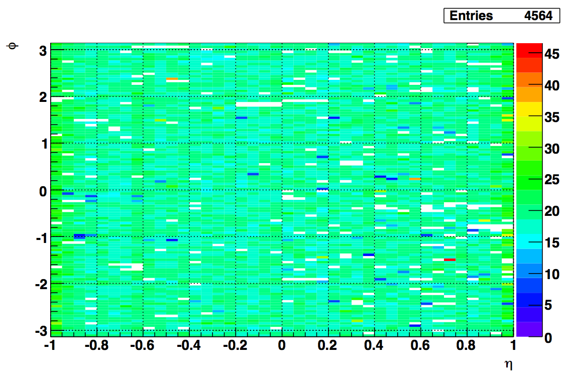
10 Electron E/p from pp500 L2W events
I ran the usual calibration code over the L2W data produced for the W measurement.
To find an enriched electron sample, I applied the following cuts to the tracks, the tower that the track projects to, the 3x3 tower cluster, and the 11 BSMD strips in both planes under the track:
central tower adc - pedestal > 2.5*rms
enter tower = exit tower
track p < 6 and track p > 1.5
dR between track and center of tower < 0.025
track dEdx > 3.4 keV/cm
bsmde or bsmdp adc total > 50 ADC
no other tracks in the 3x3 cluster
highest energy in 3x3 is the central tower
The energies were calculated using ideal gains and relative gains calculated by Joe Seele from tower slopes.
The corrections were calculated for every 2 eta rings and each crate. The corrections for each 2 rings were calculated first and then applied. The analysis was rerun, then the E/p was calculated for each crate.
The calibration constants will be uploaded to a different flavor to be used with the preliminary W analysis.
Fig. 1 E/p spectrum for all electrons
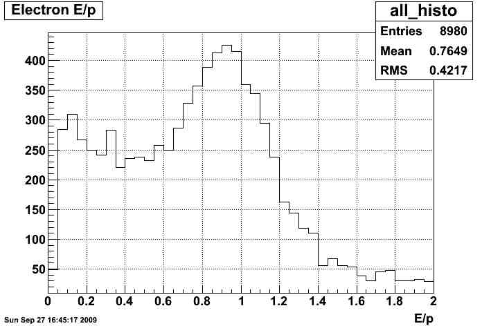
Fig. 2 p vs E/p spectrum for all electrons
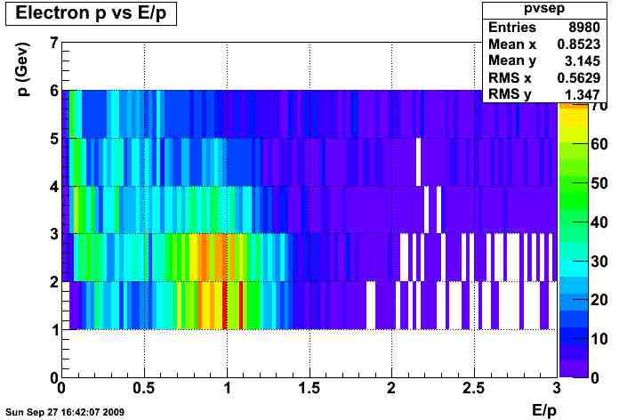
Fig. 3 BSMDP vs BSMDE for all electrons
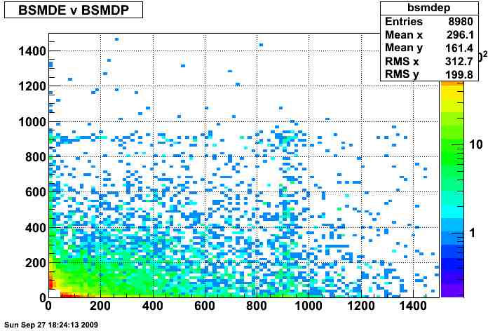
Fig. 4 corrections by eta ring
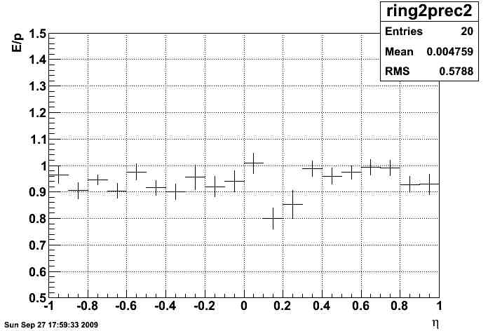
Fig. 5 Crate corrections
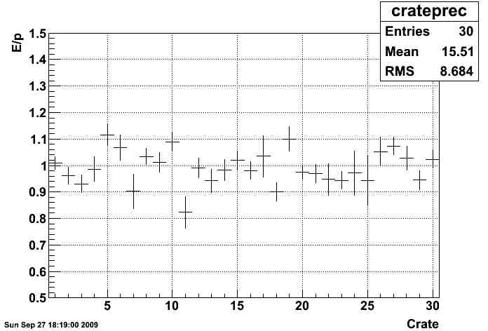
Fig. 6 difference between positrons (blue) and electrons (red):
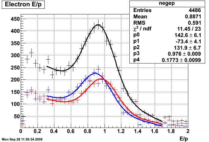
Update: I reran the code but allowed the width of the gaussian to only be in the range 0.17 - 0.175. This region agrees with almost all of the previously found widths within the uncertainties. The goal was to fix a couple fits that misbehaved. The updated corrections as a function of eta are shown below.
Fig. U1
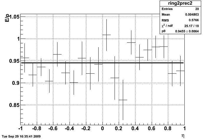
Update 09/30/2009: Added 2 more plots.
Fig. V1 East vs. West (no difference observed)
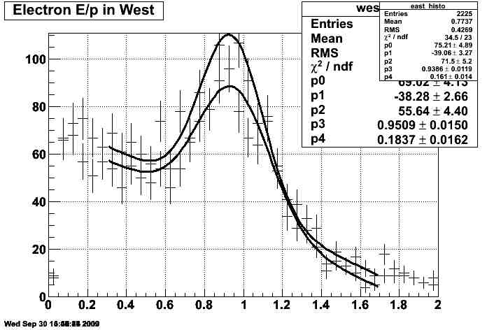
Fig. V2 slices in momentum (not much difference)
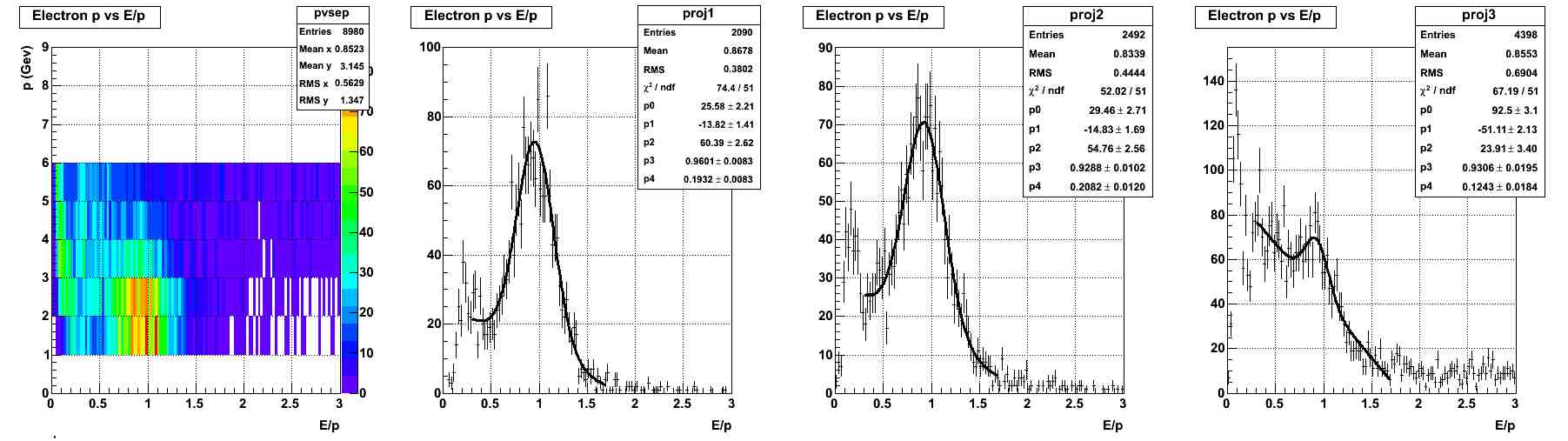
Attached are the histograms for each ring and crate.
12 Correcting Relative gains from 500 GeV L2W
After examining the Z invariant mass peak calculated using the L2W data stream with the offline calibration applied, it seemed like there was a problem. The simplest explanation was that the relative gains were reversed, so that hypothesis was tested by examining the Z peak with the data reversed.
The slopes were also recalculated comparing the original histogram to histograms corrected with the relative gains and the inverse of the relative gains.
In the following two figures, black is the original value of the slopes, red has the relative gain applied, and blue has the inverse of the relative gain applied.
Fig 1 Means of slope by eta ring with RMS
.png)
Fig 2 RMS of slope by eta ring
.png)
The E/p calculation improves after making the change to the inverse of the relative slopes because the effect of outliers is reduced instead of amplified.
Fig 3 E/p by eta ring with corrected relative gains
.png)
Update:
After last week's discussion at the EMC meeting, I recalculated all of the slopes and relative gains.
Fig 4 Update Slope RMS calculation
.png)
I then used these relative gains to recalculate the absolute calibration. Jan used the calibration to rerun the Z analysis.
Fig 5 Updated Z analysis
.png)
The updated calibration constants will now supercede the current calibration constatns.
13 Updating Calibration using the latest L2W production
I recalculated the Barrel calibration using the latest L2W production, which relies on the latest TPC calibration. It is suggested that this calibration be used to update the current calibration.
Fit Details:
Negative Peak location: 0.941
Negative Sigma: 0.14
Positive Peak location: 0.933
Positive Sigma: 0.17
<p> = 3.24 GeV
Fig 1. E/p for all electron (black), positive charged (blue), negative charged (red)
.png)
14 200 GeV Calibration
I selected 634 runs for calibration from the Run 9 production, processing over 300M events. The runs are listed in this list, with their field designation.
The MIP peak for each tower was calculated. 4663 towers had MIP peaks found. 38 were marked as bad. 99 were marked as MIPless. The MIP peak fits are here.
The electrons were selected using the following cuts:
- |vertex Z | < 60 cm
- vertex ranking > 0
- track projection enters and exits same tower
- tower status = 1
- 1.5 < track p < 10.0 GeV/c
- tower adc - pedestal > 2.5 * pedestal RMS
- Scaled dR from center < 0.02
- 3.5 < dE/dx < 5.0
- No other tracks in 3x3 cluster
- No energy in cluster > 0.5 central energy
- Track can only point to HT trigger tower if a non-HT trigger fired in the event
Fig. 1: Here is a comparison of all electrons from RFF (blue) and FF (red):
.png)
The RFF fit mean comes to 0.965 +/- 0.001. The FF fit mean comes to 0.957 +/- 0.001. The total fit is 0.957 +/- 0.0004.
Fig. 2 Comparison of electron (red) positron (blue):
.png)
Positron fit results: 0.951 +/- 0.001. Electron fit results: 0.971 +/- 0.001
Calibration was calculated using MIPs for relative calibration and absolute calibration done for eta slices by crate (30 crates, 20 eta slices per crate).
The outer ring on each side was calibrated using the entire ring.
2 towers were marked bad: 2439 2459 due to a peculiar E/p compared to the other in their crate slice. It is suggested this is due to bad bases.
Fig 3 Crate Slice E/p correction to MIPs (eta on x axis, phi on y axis):
.png)
New GEANT correction
A new geant correction was calculated using new simulation studies done by Mike Betancourt. The energy and pseudorapidity dependence of the correction was studied, and the energy dependence is small over the range of the calibration electron energies.
A PDF of the new corrections are here.
Is it statistical?
From this plot, it can be seen that most of the rings have a nonstatistical distribution of E/p values in the slices. The actual E/p values for each ring (for arbitrary slice value) can be seen here.
Comparison to previous years
Fig 4 Eta/phi of (data calibration)/(ideal calibration)
.png)
Fig 5 Eta ring average of (data calibration)/(ideal calibration)
.png)
Issues:
- FF vs RFF (partially examined)
- positive vs negative (partially examinced)
- eta/phi dependence of geant correction, direction in eta/phi
- dR dependence of calibration
- comparison to previous year
Database
These pages describe how to use the BEMC database. There is a browser-based tool that you can use to view any and all BEMC tables available at:
http://www.star.bnl.gov/Browser/BEMC/
Frequently Asked Questions
How do I use the database as it looked at a particular time?
You might be interested in this tip if e.g. you want to repeat an analysis performed before additional tables were added to the BEMC database. Add the following lines of code to your macro after St_db_Maker is instantiated, and change myDate and myTime as appropriate:
Int_t myDate = 20051231;
Int_t myTime = 235959;
dbMaker->SetMaxEntryTime(myDate,myTime);
How do I force St_db_Maker to use the event time I specify?
If you're running over simulation files, where the event timestamp is not a meaningful quantity (at least, it's not meaningful for the BEMC database), you need to choose a particular event timestamp that best represents the state of the BEMC during the data-taking period to which you're comparing the simulations. A list of timestamps is being compiled at Simulation Timestamps. Add the following lines of code to your macro, and change myDate and myTime as appropriate:
Int_t myDate = 20051231;
Int_t myTime = 235959;
dbMaker->SetDateTime(myDate,myTime);
Calibrations Database
All calibration information is stored in the STAR database. We have the following tables for BEMC calibrations:- For the BTOW and BPRS detectors:
- St_emcCalib - this table contains absolute gain information for each channel
- St_emcPed - this table contains pedestal values for each channel
- St_emcGain - this table contains a gain correction factor vs. time for each channel (not currently used)
- St_emcStatus - this table contains the final status for each channel
- For the BSMDe and BSMDp detectors:
- St_smdCalib - this table contains absolute gain information for each channel
- St_smdPed - this table contains pedestal values for each channel
- St_smdGain - this table contains a gain correction factor vs. time for each channel (not currently used)
- St_smdStatus - this table contains the final status for each channel
To get a pointer for those tables in an analysis maker do:
TDataSet *DB = GetInputDB("Calibrations/emc/y3bemc"); // for towers

St_emcCalib *table = (St_emcCalib*) DB->Find("bemcCalib");
emcCalib_st *struct = table->GetTable();
Important Information About Pedestal Tables
In order to save space and make the download faster, PEDESTALS and RMS are saved as SHORT. So, the real pedestal value is PED/100. Similarly, in order to save tables in the database you have to multiply the real pedestal by 100. The same goes for the RMS.SMD has different pedestals for different capacitors. Only 3 pedestal values are saved:
- Pedestal 0 is the average of 126 capacitors
- Pedestal 1 is the pedestal value for capacitor 124
- Pedestal 2 is the pedestal value for capacitor 125
unsigned char cap = (char) rawHit->calibrationType();
if(cap > 127) mCap[i][did-1]-=128;
Status Information
The St_emcStatus and St_smdStatus tables contain final status codes for each tower. The final status is a combination of installation/run status, pedestal status and calibration status. The final status has a bit pattern as follows:- 0 - not installed
- 1 - installed / running
- 2 - calibration problem
- 4 - pedestal problem
- 8 - other problem (channel removed, dead channel, etc.)
To check individual bits of the final status do
- (status&1) == 1 means tower is installed
- (status&2) == 2 means a calibration problem
- (status&4) == 4 means a pedestal problem
- (status&8) == 8 means another problem
Tables Structure
/*    emcCalib.idl
*
*  Table: emcCalib
*
*       description: //:  Table which contains all calibration information
*/
struct emcCalib {
   octet  Status[4800];      /* status of the tower/wire (0=problem, 1=ok)  */
   float  AdcToE[4800][5];   /* ADC to Energy  */
};
/*    emcPed.idl
*
*  Table: emcPed
*
*       description: *    //:  Table which contains pedestal information for emctower ADCs
*/
struct emcPed {
   octet  Status[4800];           /* status of the emc tower(0=problem, 1=ok)  */
   short  AdcPedestal[4800];      /* ADC pedestal of emc tower x 100  */
   short  AdcPedestalRMS[4800];   /* ADC pedestal RMS of emc tower x 100  */
   float  ChiSquare[4800];        /* chi square of Pedestal fit */
};
/*    emcGain.idl
*
*  Table: emcGain
*
*       description: //:  Table which contains gain correction information
*/
struct emcGain {
   octet  Status[4800];   /* status of the tower/wire (0=problem, 1=ok)  */
   float  Gain[4800];     /* Gain Variation  */
};
/*    emcStatus.idl
*
*  Table: emcStatus
*
*       description: //   which emc towers are up and running
*/
struct emcStatus {
   octet  Status[4800];   /*   */
};
/*    smdCalib.idl
*
*  Table: smdCalib
*
*       description: //:  Table which contains all calibration information
*/
struct smdCalib {
   octet  Status[18000];      /* status of the tower/wire (0=problem, 1=ok)  */
   float  AdcToE[18000][5];   /* ADC to Energy  */
};
/*    smdPed.idl
*
*  Table: smdPed
*
*       description: *    //:  Table which contains pedestal information for shower max ADCs
*/
struct smdPed {
   octet  Status[18000];            /* status of the smd stripe (0=problem,1=ok)  */
   short  AdcPedestal[18000][3];    /* ADC pedestals of smd strip x 100  */
   short  AdcPedestalRMS[18000][3]; /* ADC pedestals RMS of smd strip x 100  */
};
/*    smdGain.idl
*
*  Table: smdGain
*
*       description: //:  Table which contains gain information
*/
struct smdGain {
   octet  Status[18000];   /* status of the tower/wire (0=problem, 1=ok)  */
   float  Gain[18000];     /* Gain Variation  */
};
/*    smdStatus.idl
*
*  Table: smdStatus
*
*       description: //   which smds are up and running
*/
struct smdStatus {
   octet  Status[18000];   /*   */
};
Control Room
We use a crontab on emc01.starp.bnl.gov to update the trigger database tables as well as the "offline" pedestals throughout the run. Here's the relevant portion of /etc/crontab:00 4 * * * emc /home/emc/online/emc/pedestal/job
00 * * * * emc /home/emc/online/emc/trigger/job
10 * * * * emc /home/emc/online/emc/trigger/job
20 * * * * emc /home/emc/online/emc/trigger/job
30 * * * * emc /home/emc/online/emc/trigger/job
40 * * * * emc /home/emc/online/emc/trigger/job
50 * * * * emc /home/emc/online/emc/trigger/jobPedestal Job
The job runs every day at 4:00 AM and executes the script$EMCONLINE/pedestal/updateOnlinePed
which in turn calls the root4star macro
$EMCONLINE/pedestal/makeOnlinePed.C
This macro calculates pedestals for all 4 subdetectors and uploads the tables to the STAR database. A local backup copy of each table is stored in
$EMCONLINE/pedestal/tables/tables/
Trigger Job
The job runs $EMCONLINE/trigger/updateTriggerDB every ten minutes. If the file $EMCONLINE/trigger/RUNMODE contains STOP, the job will do nothing. $EMCONLINE/trigger/startTriggerDB and $EMCONLINE/trigger/stopTriggerDB can be used to change the content of RUNMODE. The updateTriggerDB shell script contains some decent documentation which I've reproduced here:# this script checks if ANY of the BEMC trigger
# configuration had changed. If so, it updated the
# database with the new trigger configuration
#
# it runs as a cronjob every 5-10 minutes in the star01
# machine
#
# this script follows the steps bellow
#
# 1. check the file RUNMODE. If content is STOP, exit the
# program. This is done if, for some reason, we
# want to stop the script from updating the DB
#
# 2. SCP the config_crate* and pedestal_crate* files
# from sc3.starp.bnl.gov machine
#
# 3. SCP the trigegr masks from startrg2.starp.bnl.gov machine
#
# 4. Copy these files to the sc3 and startrg2 directories
#
# 5. Compare these files to the files saved in the sc3.saved
# and startrg2.saved directories
#
# 6. If there is no difference, clear the sc3 and startrg2
# directories and exit
#
# 7. If ANY difference was found, copy the contents of the
# sc3 and startrg2 directories to sc3.saved and startrg2.saved
# Also saves the directory with timestamped names in the
# backup directory
#
# 8. runs the root4star macro that create the tables from
# the files in those directories and save them to the DB
# It also creates plain text file bemcStatus.txt with the same information
# for the trigger people and Pplots
#
# 9. clear the sc3 and startrg2 directories and exit
#
# you can also run it by hand with the command
#
# updateTriggerDB TIMESTAMP FORCE
#
# where TIMESTAMP is on the format
#
# YYYYMMDD.hhmmss
#
# if FORCE = yes we force saving the DB
#
# this procedure overwrites the RUNMODE variable
#
# AAPSUAIDE, 12/2004
#Basically the job is always checking for changes to the trigger pedestals, status tables, and LUTs and uploaded a new table if any changes are found.
Mapping DB Proposal
Proposal
We propose to add a new set of tables to the Calibrations_emc database that will track the electronics mapping for the BEMC, BSMD, and BPRS and allow for an alternative implementation of StEmcDecoder.
Motivation
The existing BEMC electronics mapping code (StDaqLib/EMC/StEmcDecoder) has become difficult to maintain. Each time we discover something about the BEMC that requires an update to our lookup tables we have to decipher the algorithms that generate these lookup tables, and more often than not our first guess about how to add the new information is wrong.
StEmcDecoder is also inefficient because it doesn’t track the validity range of the current lookup tables and so it rebuilds the tables every event. Analysis jobs spend a non-neglible amount of CPU time rebuilding these decoder tables.
The information in the decoder is critical for BEMC experts, but the interface to that information is less than ideal. StEmcDecoder does not even have CINT bindings. An SQL interface would allow for much easier debugging.
For the End User
We are preserving the StEmcDecoder interface and reimplementing it to use the DB tables. Offline users should see a seamless transition. StEmcDecoder also plays an important role in the online p-plots. We’ll need to find a solution that allows access to the DB tables in that framework.
For Experts
The new mapping tables will contain a row for each detector element, so we expect that querying the tables using SQL will prove to be a valuable debugging tool. A simplified query might look like:
SELECT elementID,m,e,s FROM bemcMapping WHERE triggerPatch=5 and beginTime='2007-11-01 00:00:00';
which would yield
+-----------+------+------+------+
| elementID | m    | e    | s    |
+-----------+------+------+------+
|      1709 |   43 |    9 |    2 |
|      1710 |   43 |   10 |    2 |
|      1711 |   43 |   11 |    2 |
|      1712 |   43 |   12 |    2 |
|      1729 |   44 |    9 |    1 |
|      1730 |   44 |   10 |    1 |
|      1731 |   44 |   11 |    1 |
|      1732 |   44 |   12 |    1 |
|      1749 |   44 |    9 |    2 |
|      1750 |   44 |   10 |    2 |
|      1751 |   44 |   11 |    2 |
|      1752 |   44 |   12 |    2 |
|      1769 |   45 |    9 |    1 |
|      1770 |   45 |   10 |    1 |
|      1771 |   45 |   11 |    1 |
|      1772 |   45 |   12 |    1 |
+-----------+------+------+------+
16 rows in set (0.12 sec)
Previously, we needed to write one-off compiled programs to export this kind of information out of the decoder.
Draft IDLs
struct emcMapping {
   octet m;                     /* module 1-120 */
   octet e;                     /* eta index 1-20 */
   octet s;                     /* sub index 1-2 */
   unsigned short daqID;        /* ordering of elements in DAQ file 0-4799 */
   octet crate;                 /* electronics crates 1-30 */
   octet crateChannel;          /* index within a crate 0-159 */
   octet TDC;                   /* index in crate 80, 0-29 */
   unsigned short triggerPatch; /* tower belongs to this TP 0-299 */
   octet jetPatch;              /* tower belongs to this JP 0-11 */
   unsigned short DSM;          /* just integer div TP/10 0-29 */
   float eta;                   /* physical pseudorapidity of tower center */
   float phi;                   /* physical azimuth of tower center */
   char comment[255];
}
struct smdMapping {
octet m; /* module 1-120 */
octet e; /* eta index 1-150 (eta), 1-10 (phi) */
octet s; /* sub index 1 (eta), 1-15 (phi) */
octet rdo; /* readout crate 0-7 */
unsigned short rdoChannel; /* index in crate 0-4799 */
octet wire; /* wire number 2-80 */
octet feeA; /* A value for FEE 1-4 */
float eta; /* physical pseudorapidity of strip center */
float phi; /* physical azimuth of strip center */
char comment[255];
}struct prsMapping {
octet m; /* module 1-120 */
octet e; /* eta index 1-20 */
octet s; /* sub index 1-2 */
octet PMTbox; /* PMT box 1-30 (West), 31-60 (East) */
octet MAPMT; /* MAPMT # for this element in PMTbox 1-5 */
octet pixel; /* index inside MAPMT 1-16 */
octet rdo; /* readout crate 0-3 */
unsigned short rdoChannel; /* index in readout crate 0-4799 */
octet wire; /* wire number 1-40 */
octet feeA; /* A value for FEE 1-2 */
octet SCA; /* switched capacitor array 1-2 */
octet SCAChannel; /* index inside SCA 0-15 */
octet powerSupply; /* 1-2 */
octet powerSupplyModule; /* 1-15 */
octet powerSupplyChannel; /* 0-14 */
float eta; /* physical pseudorapidity of tower center */
float phi; /* physical azimuth of tower center */
char comment[255];
}I also proposed MySQL schemata on my blog, but I guess in STAR these IDLs define the schema.
Performance Estimates
I’ve temporarily installed tables on our MIT mirror and filled them with data describing the 2008 BEMC electronics mapping. Here are the stats:
*************************** 1. row ***************************
           Name: bemcMapping
         Engine: MyISAM
        Version: 10
     Row_format: Dynamic
           Rows: 4800
 Avg_row_length: 55
    Data_length: 268732
Max_data_length: 281474976710655
   Index_length: 163840
      Data_free: 0
 Auto_increment: 4801
    Create_time: 2008-11-14 16:03:51
    Update_time: 2008-11-14 16:05:45
     Check_time: NULL
      Collation: latin1_swedish_ci
       Checksum: NULL
 Create_options:
        Comment:
*************************** 2. row ***************************
           Name: bprsMapping
         Engine: MyISAM
        Version: 10
     Row_format: Dynamic
           Rows: 4800
 Avg_row_length: 70
    Data_length: 336036
Max_data_length: 281474976710655
   Index_length: 165888
      Data_free: 0
 Auto_increment: 4801
    Create_time: 2008-11-14 17:52:53
    Update_time: 2008-11-14 17:59:40
     Check_time: 2008-11-14 17:52:53
      Collation: latin1_swedish_ci
       Checksum: NULL
 Create_options:
        Comment:
*************************** 3. row ***************************
           Name: bsmdeMapping
         Engine: MyISAM
        Version: 10
     Row_format: Dynamic
           Rows: 18000
 Avg_row_length: 52
    Data_length: 936000
Max_data_length: 281474976710655
   Index_length: 604160
      Data_free: 0
 Auto_increment: 18001
    Create_time: 2008-11-14 16:03:51
    Update_time: 2008-11-18 01:48:36
     Check_time: NULL
      Collation: latin1_swedish_ci
       Checksum: NULL
 Create_options:
        Comment:
*************************** 4. row ***************************
           Name: bsmdpMapping
         Engine: MyISAM
        Version: 10
     Row_format: Dynamic
           Rows: 18000
 Avg_row_length: 52
    Data_length: 936000
Max_data_length: 281474976710655
   Index_length: 604160
      Data_free: 0
 Auto_increment: 18001
    Create_time: 2008-11-14 16:03:51
    Update_time: 2008-11-18 02:13:36
     Check_time: NULL
      Collation: latin1_swedish_ci
       Checksum: NULL
 Create_options:
        Comment:
4 rows in set (0.11 sec)
This information is supposed to be static, even from year-to-year. In reality, we discover some details about the mapping each year which will require updates to some of these rows. There should certainly be no intra-run changes, so StEmcDecoder will need to retrieve 4800+4800+18000+18000 rows from the DB for each BFC and user job.
The equivalent C++ array sizes (excluding the comment field as I’m not sure how its handled) will be 101 KB (4800*21) for BEMC, 115 KB (4800*24) for BPRS and 288 KB (18000*16) for each SMD plane.
Pedestals / Status Tables
Code for the calculation of the BTOW & BSMD status tables has been made publicly accessible. BTOW status code is in StRoot/StEmcPool/CSMStatusUtils. The following studies of pedestals and status tables have been performed:
BTOW
2006
Dave S. - status
2004
Thorsten - 62 GeV AuAu status tables
Oleksandr - 200 GeV AuAu pedestals
Oleksandr - 62 GeV AuAu pedestals
2003
Oleksandr - dAu status tables
Oleksandr - pp status tables
BSMD & BPSD
2006
Priscilla - SMD pedestals
2005
Frank - SMD status for pp (bug found in code http://rhig.physics.yale.edu/~knospe/cucu200/bsmd_status_bug.htm)
Frank's code used to generate status tables from MuDsts
2004
200 GeV AuAu SMD status - taken by Martijn
Marcia - 200 GeV AuAu SMD pedestals
Subhasis - 62 GeV AuAu SMD & PSD pedestals
2003
Martijn - dAu SMD status
CSMStatusUtils
This is CSMStatusUtils, which outputs the status of either calorimeter to text and root status files. Documentation is by Dave Relyea. The code can be found atStRoot/StEmcPool/CSMStatusUtils
History:
I was given code from both Joanna and Thorsten to figure out the status of the calorimeter towers over all pp production runs. I merged the two sets of code, and and created a package called CSMStatusUtils.
Method:
The first piece of code in CSMSU takes every run and fills a 2-d histogram of ALL channels vs hit number (in ADC counts, from 0 to 150). A second routine then combines these histograms from run subsets into single histograms for each run. From the second routine and on down, the EEMC and BEMC are done entirely separately; the code needs to be run twice, once for each detector.
The code has an algorithm which then takes runs in each fill and combines them until the average number of hits above pedestal for all channels is greater than 100. If runs are left over at the end of a fill, their statistics are added to prior runs in the fill.
For each combined set of runs, the code puts each channel through a series of tests. It finds the pedestal (and writes it out to a file, btw) and determines if the pedestal is abnormally wide, or whether it falls outside acceptable limits (ADC channels 0 to 3, or 147 to 150). It compares all towers' mean number of hits (ten sigma) above pedestal, and then flags towers which have 10x as many hits as the average, or 40x fewer. Finally, it looks for stuck bits (either on or off) in the 1, 2, 4, or 8 position, and flags channels with stuck bits.
The code writes out a table (in text format) for each set of runs with the status of each channel clearly marked. This table is also written in ROOT format, to be read by existing BEMC algorithms. Also written is a hot tower plot, so the hot tower results can be eyeballed. The code can also write out gif files of the spectra of every channel that failed a status test, so long as the number of channels in a given run set that failed the test is less than 25 (**for 2004 pp, gif files were not written out**). Finally, the code creates a nice html file containing links to html subfiles detailing the channel status for each run set, which in turn link to the gif files.
As a final step, the code takes the text files and creates a new series of text status files with the results in differential format, meaning channels whose status didn't change from run set to run set are omitted. However, since some channels fall very near the thresholds of certain status tests (for instance, channels whose pedestals sit at 2.9 ADC counts), I make the requirement that the channel's status must not have changed more than ten percent of the time over all runs sets, excluding runs in which all channels were bad (for nominal production running, this needs to be done, of course!). If it has, it is marked bad once at the beginning, and then does not appear in any of the differential files.
************************************************************************
Running:
To run CSMSU, the first step is to use the FileCatalog to create a list of all the files you wish to analyze. The command I use is typically something like:
get_file_list.pl -keys 'path,filename' -cond 'production=P04ik,tpc=1,emc=1, trgsetupname=productionPP||productionPPnoEndcap||pp||PP,filename~st_physics,filetype=daq_reco_mudst' -onefile -limit 100000 -distinct > allthephysicsfiles
Note that the output format I use is just 'path,filename', and I keep the :: delimiter that the FileCatalog uses. My next step is to call
CSMSU/scripts/analysis0 allthephysicsfiles
(YOU NEED TO CHANGE THE HEADER IN THIS FILE TO YOUR OWN OUTPUT DIRECTORY)
which takes the "allthephysicsfiles" file from FileCatalog, splits it up into groups of 20 miniruns, and submits the entire processing job to batch. Note - if I knew how to use the XML submission scripts, I would, but the online documentation for them doesn't mention how to code up your macro (.C) file such that the XML header file will work. No matter.PLEASE NOTE: Each minirun will generate about a 200k file. This adds up to ENORMOUS disk space for large runs. The 2004 pp run takes up about 1.4 Gig. The 2004 Au-Au run would be even larger. Thus, I really need to learn how to
use the XML submission scripts.
(FROM HERE ON, SCRIPT FILES CALL MACROS IN THE MACROS DIRECTORY. YOU NEED TO CHANGE THE DEFAULT ARGUMENTS OF THE MACROS TO YOUR WORKING DIRECTORY. YOU CAN DO THIS IN THE SCRIPT, OR JUST MAKE YOUR OWN SCRIPT, SINCE THEY'RE ALL TRIVIAL ONE LINE SCRIPTS ANYWAY. SORRY ABOUT THE CAPS.)
After all miniruns have been processed, the next step is to combine them into runs. The script "analysis1" does this.Next, you want to run the actual status code on the files. The script "analysis2" does this. PLEASE NOTE: this macro requires an x window, as root needs to be able to Draw certain things. I don't know how to do this in batch,
so I always run this interactively. It's not a good solution, but for now, it's a solution.
Finally, you want to generate the ".root" status files and the concatenated status files (to alert you to changes in calorimeter tower status). The script "analysis3" does this.
StBSMDStatusMaker
This page gives a brief overview of the code Frank Simon developed to create SMD Status Tables from MuDSTs.
Some features and limitiations of the code:
- Create one status table per fill for each SMD plane (if enough statistics are available)
- all triggers are used to maximize statistics (this can be a potential problem if there are hot trigger towers)
- pedestals are taken from the data base (MuDST SMD data are zero-suppressed)
- db-readable status tables can be created. Currently there are only to status flags implemented: good and bad. Adding more "variety" is straigth forward
- can be used with the STAR scheduler, no specific ordering of the input files required (although some structure in the job submission is recommended, see below)
Basic ideas behind the code:
- based on Daves tower status code, but: there are some very important differences
- One job runs over several MuDST files, when a new fill number is encountered, a new output file is opened. That way, the jobs can be run with the STAR scheduler and they can use files on distributed storage, since no particular ordering of the input files is needed
- for each fill, a file with 18000 channel TH2Fs storing amplitude information for each SMD channel is created (this method of dealing with random file order is a bit disk space hungry, so make sure enough space is available (~ 10 GB for 2005 pp); this can be deleted after the next step), other information such as time stamps and pedestals are stored in text files
- As a next step, the large number of files created by jobs on MuDSTs is consolidated into one file per fill
- Status tables are created from each of those files (one per fill, if statistics are sufficient, otherwise no status table for that fill is created)
- db readable files are produced from these status tables
Running the code
- Copy and compile the code in StRoot/StBSMDStatusMaker
- Copy the macro that runs the code: RunStatus.C
- Create scheduler scripts to submit your jobs. For pp2005, 50 jobs per job seems to give jobs with useful runtimes. In order to not get a totally randomized fill distribution in your jobs, submit them by day. A macro that creates a .csh that you can use to submit jobs by day is CreateSubmitScript.C, a template job describtion (you have to modify tha paths to suit your needs) is pp2005Template.xml
- Submit your jobs
- Once all jobs are done, create a list of all output files via ls * > FileList.list in the directory where your output ended up
- Consolidate data using the file list: run macro DoAdding.C after compiling AddHistograms.C (via .L AddHistograms.C++), this macro takes the directory where the files are located and the file list as arguments. This creates three files per fill: Fill*.root containing the histograms, Fill*.ped containing pedestal db information and Fill*.time containing the (approximate) start time of the fill
- Create a list of root files via ls Fill*.root > FileList.list and convert it into a list of fill numbers using the macro GetListOfFills.C. This maco takes the file list and a file name for the fill number list as argument
- Perform the status table creation. For that, compile the shared library StatusTools.C (via .L StatusTools.C++), then run the macro ProcessList.C, with arguments RunList (created previously) and the directory where the Fill* files are located. The output of this is a number of files per fill (root file, flag file and time stamp file). The flag and the time stamp file are needed to create the db readable status table, the root file contains histograms created during the analysis process.
- Create db readable status tables. This is done by running the macro WriteStatusFiles.C. This takes the directory where the flag and timestamp files are located as an argument. Two important notes:
- This macro needs the full STAR environment (all other steps above except the running of jobs can be done on standalone machines)
- The order in which the flag and time files are written (created) is crucial, since gSystem->GetDirEntry() is used to loop over all files. So care has to be taken if the files are copied from somewhere else
- Copy the db readable files to the database location in StarDb, and test them! Use TestStatusFiles.C for example.
For questions, please don't hesitate to contact me at fsimon@mit.edu!
Simulation Timestamps
All 4800 perfect:dbMaker->SetDateTime(20070101,000001);
Run 5 pp, selected by Spin PWG:
dbMaker->SetDateTime(20050506,214129);
some more info from Frank on detailed SMD status:
if (dbTime == 1) db1->SetDateTime(20050423,042518); //2005 stat1
else if (dbTime == 2) db1->SetDateTime(20050521,100745); //2005 stat2
else if (dbTime == 3) db1->SetDateTime(20050529,210408); //2005stat3
else db1->SetDateTime(20050610,120313); //2005, JumbodbMaker->SetDateTime(20060522,112810);
Table Insertion Timeline
This page keeps a log book of all the BEMC database modifications. Please use this information in order to make sure about the version of the tables you are grabbing from DATABASE. The table is sorted by EntryTime.
If you'd like to run an analysis using the database as it looked at some particular time, use the method
St_db_Maker *dbMaker = new St_db_Maker("StarDb", "MySQL:StarDb");
Int_t myDate = 20051231;
Int_t myTime = 235959;
dbMaker->SetMaxEntryTime(myDate,myTime);
You can use the BEMC DB Browser to look at all the tables in the database
| row number |
EntryTime | Tables | Note |
| 1 | 2005-11-03 | pp2005 bemcCalib table with timestamp = 2005-03-22 00:00:01 was uploaded to the database |
Adam's calibration table for pp2005. Click here for details |
| 2 | 2005-12-07 | pp2005 offline bemcStatus with timestamp between 2005-04-19 11:36:11 and 2005-06-24 08:58:25 were uploaded to the database |
Dave's status tables for the pp2005 run |
| 3 | 2006-02-08 | pp2005 online bemcPed with timestamp between 2005-04-19 05:37:10 and 2005-06-10 23:38:20 were deactivated |
Corruption problems reported by Dave |
| 4 | 2006-02-09 | pp2005 offline (Dave's) bemcPed with timestamp between 2005-04-19 05:37:10 and 2005-06-10 23:38:20 were uploaded to the database |
Replacement for pp2005 bemcPed tables |
| 5 | 2006-02-09 | pp2004 online bemcPed with timestamp between 2004-05-05 01:41:40 and 2004-05-14 23:21:19 were deactivated |
Bad tables reported by Joanna with large RMS values and missing channels. Click here for details |
| 6 | 2006-02-09 | pp2004 offline (Dave's) bemcPed with timestamp between 2004-05-05 01:41:40 and 2004-05-14 23:21:19 were uploaded to the database |
Replacement for pp2004 bemcPed tables |
| 7 | 2006-02-22 | AuAu and pp 2004 bemcCalib table with timestamp 2004-01-01 00:04:00 was uploaded to database |
Improvements in calibration by Adam Kocoloski. Click here for details |
| 8 | 2006-02-22 | CuCu 2005 bemcCalib table with timestamp 2005-02-01 00:00:01 was uploaded to database |
Improvements in calibration by Adam Kocoloski. Click here for details |
| 9 | 2006-02-22 | pp 2005 bemcCalib table with timestamp 2005-03-22 00:00:02 was uploaded to database |
Improvements in calibration by Adam Kocoloski. Click here for details This is a copy of the table saved in row number 8. This is necessary because there were calibration tables saved for pp2005 run |
| 10 | 2006-03-07 | Saved perfect status tables (bemc, bsmde, bsmdp and bprs) for run 6 with timestamp 2006-01-01 00:00:00 |
First order status tables necessary for fast production and pp2006 vertex finder |
| 11 | 2006-03-30 | Saved initial BTOW calibration for pp2006 with timestamp 2006-03-11 08:27:00 |
First calibration for pp2006 (online). Based on eta-slices MIP peaks and slopes equalization. Click here for details |
| 12 | 2006-04-19 | A set of perfect status tables (bemc, bsmde, bsmdp and bprs) was saved in DB for the CuCu2005 with timestamp 2005-01-01 00:00:00 |
This makes sure that the 2004 status tables are not picked for any analysis/production done with the 2005 CuCu data while there is no detailed status tables available |
| 13 | 2006-04-20 | A perfect status table for BTOW, including only the west side of the EMC was saved in DB for the CuCu2005 with timestamp 2005-01-01 00:00:01 |
Added to replace previous perfect status table that includes the full detector because the east side was being commissioned |
| 14 | 2006-06-16 | Offline BSMD status tables for 2005 pp running. Event timestamps are between 2005-04-16 06:48:09 and 2005-06-23 19:38:42 |
Tables produced by Frank Simon. Click here for details |
| 15 | 2006-06-21 | Offline BTOW status tables for 2005 pp running. Event timestamps are between 2005-04-19 11:36:11 and 2005-05-14 09:17:59 |
These tables should have been / were uploaded back in row 2. It's not clear what happened to them. |
| 16 | 2006-06-21 | Online BTOW pedestals for 2006 pp running. Event timestamps are between 2005-03-02 08:40:15 and 2005-06-19 04:41:18 |
BTOW pedestals were calculated and saved to the DB automatically during the run. Unfortunately the tables were corrupted during the upload, so we need to upload these tables again with +1 second timestamps. |
| 17 | 2006-08-15 |
BSMD pedestals for Run 6. |
Details |
| 18 | 2006-08-16 |
BTOW status for Run 6. |
~1 table/fill. Should be good enough for vertex finding during production, but not necessarily the final set of tables. Details |
| 19 | 2006-10-17 |
Perfect BPRS status table for 2006 run |
Begin time 2006-01-01 |
| 20 | 2006-11-10 | BTOW status for Run 5 CuCu |
Link needs to be updated with a summary page. Details |
| 21 | 2006-11-21 |
Fixed timestamps for Run 5 pp status |
See starsoft post |
| 22 | 2006-11-30 |
Fixed timestamps for Run 5 pp peds |
See starsoft post |
| 23 | 2006-12-07 | Offline BTOW calibration for Run 6 | Run 6 BTOW Calibration |
| 24 | 2007-01-17 | Final BTOW status tables for trans,long2 | Details |
| 25 | 2007-02-13 | Corrected 3 Run6 tower peds in few runs | Hypernews discussion |
| 26 | 2007-02-26 | Final BSMD Run6 status tables | Details |
Trigger Database
This database stores all BEMC trigger information such as trigger status, masks and pedestals used to obtain the high tower and patch sum information. The database is updated online while taking data. We have the following table formats:- St_emcTriggerStatus - this table contains status/mask information for the trigger
- St_emcTriggerPed - this table contains the pedestal and bit conversion scheme used in the trigger
- St_emcTriggerLUT - this table contains the lookup table information. Because the LUT is very large it is encoded in simple formulae. The FormulaTag entry specifies the formula used for each patch.
TDataSet *DB = GetInputDB("Calibrations/emc/trigger");

St_emcTriggerStatus *table = (St_emcTriggerStatus*) DB->Find("bemcTriggerStatus");
emcTriggerStatus_st *struct = table->GetTable();
Important Information About Pedestal Tables
In order to save space and make the download fast, PEDESTALS and RMS are saved as SHORT. So, the real pedestal value is PED/100. Similarly, in order to save tables in the database you have to multiply the real pedestal by 100. The same goes for the RMS.The pedestal table also includes the 6-bit conversion scheme used to generate the high tower and patch sum information.
Status Information
The St_emcTriggerStatus table contains the status information for each single tower, high tower and patch sum (patch sum is the sum in the 4x4 patches. It is *not* the jet patch). The status is a simple 0/1 that reflects the masks that are being applied to the electronicss where- 0 - masked out
- 1 - included in trigger
Tables Structure
/*
*
*  Table: emcCalib
*
*       description: //:  Table which contains the trigger masks
*/
struct emcTriggerStatus
{
  octet PatchStatus[300];     // Patch sum masks. the index is the patch number
  octet HighTowerStatus[300]; // High tower masks. the index is the patch number
  octet TowerStatus[30][160]; // Single masks. the indexex are the crate number and position in crate
};
/*
*
*  Table: emcTriggerPed
*
*       description: *    //:  Table which contains pedestal information and 6 bits conversion used in trigger
*/
struct emcTriggerPed
{
  unsigned long PedShift; // pedestal shift
  unsigned long BitConversionMode[30][10]; // 6 bits conversion mode. the indexex are the crate number and position in crate
  unsigned long Ped[30][160]; // pedestal value. the indexex are the crate number and position in crate
};
/*
*
*  Table: emcTriggerLUT
*
*       description: *    //:  Table which contains each patch LUT information
*/
struct emcTriggerLUT
{
  unsigned long FormulaTag[30][10]; // formula tag for each [crate][patch]
  unsigned long FormulaParameter0[30][10]; // Parameter 0 for the LUT formula in [crate][patch]
  unsigned long FormulaParameter1[30][10]; // Parameter 1 for the LUT formula in [crate][patch]
  unsigned long FormulaParameter2[30][10]; // Parameter 2 for the LUT formula in [crate][patch]
  unsigned long FormulaParameter3[30][10]; // Parameter 3 for the LUT formula in [crate][patch]
  unsigned long FormulaParameter4[30][10]; // Parameter 4 for the LUT formula in [crate][patch]
  unsigned long FormulaParameter5[30][10]; // Parameter 5 for the LUT formula in [crate][patch]
};
BEMC Online Trigger Monitoring
During data taking the BEMC trigger information is monitored, and changes in the configuration (new pedestals, masks, etc.) are recorded. The code relevant to this online trigger monitoring was developed by Oleksandr, and is checked into CVS here (usage instructions in the README file). The scripts execute via a cronjob on the online machines on the starp network. In particular, there exists directories with results from previous years at /ldaphome/onlmon/bemctrgdb20XX/ on onl08.starp.bnl.gov.
The final location for this information is in the offline DB, and the definitions for the tables are given here. These DB tables are used by the StBemcTriggerSimu in the StTriggerUtilities package to replicate the BEMC trigger conditions for a particular timestamp.
The DB tables can be uploaded while taking data or stored in ROOT files to be uploaded after data taking is complete. To upload all the tables stored in ROOT files during data taking only a simple script is needed employing StBemcTablesWriter to read in a list of files and upload their information to the DB. This script (uploadToDB.C) is checked into the macros directory of in CVS here.
Yearly Timestamp Initialization
Yearly Timestamp Initialization
This page will document the yearly timestamp initialization requested by the S&C group (Run 12 for example). The purpose is to set initial DB tables for "sim" and "ofl" flavor in sync with the geometry timeline for each year. The geometry timeline is documented here.
The timestamps chosen for BEMC initialization are in the table below
| Simulation | Real Data | |
| Run 10 | 2009-12-12 | 2009-12-25 |
| Run 11 | 2010-12-10 | 2010-12-20 |
| Run 12 | 2011-12-10 | 2011-12-20 |
The "sim" tables used for initialization are ideal gains, pedestals and status tables.
The "ofl" tables used for initialization are the best known gains from previous years, and a reasonable se of pedestals and status tables from a previous year. Obviously they will be updated once the run begins and better known values are available.
To simplify the initialization process from year to year, a macro (attached below) was written which copies DB tables from previous years to the current initialization timestamp.
Hardware
BEMC_FEE_Repairs (BSMD)
Here (below) are the BSMD FEE repair record spreadsheets from Phil Kuczewski.
The one with label "BEMC_FEE_Repairs-2010.xls" is most recent, including repairs in 2010
(although on 9/8/10 Oleg says that 1 more SAS was already replaced and there likely will be 2 more)
Mapping
Information about how the BEMC detectors are indexed (Pre run14)
Oleksandr's Spreadsheet of Towers' Layout (Excel)
Oleksandr's Spreadsheet of Towers' Layout (PDF)
For run 14 there were signal cable swaps for PMT boxes 13->14, 15->16, and 45->46. The updated tower maps are here:
Run14 Tower Layout (Excel)
Run14 Tower Layout (PDF)
In these new spreasheets, the yellow, light blue, and light gray boxes are where the swaps are. On the outsides, the PMT boxes are labeled (PMB) and you can clearly see the swaps. As an example, here's how it would work:
Soft Id's 3521, 3522, 3523, 3524, ...., 3461, 3462, 3463, 3464 were swapped with
3441, 3442, 3443, 3444, ...., 3381, 3382, 3383, 3384
BSMDE 2010 mapping problem and solution
All the details of the mapping problem can be found in this ticket. This page is a summary of the problem, solution, and the implementation.
During Run 10 a problem with the BSMD mapping was discovered (details here). It was decided to continue taking data with the 2 fibers swapped for future running, and simply correct the mapping in the DB to reflect the hardware configuration before production. The mapping for the BSMD phi plane (BSMDP) was corrected (completely swapped 2 fibers in the DB) before produvtion to match the Run 10 hardware configuration, so there were no problems with BSMDP mapping in production.
Problem:
The correction to the BSMD eta plane (BSMDE) mapping, however, was incomplete and did not swap the 2 fibers in the DB completely. Ahmed found this mapping problem in "Phase I" of the 200GeV QM production (production series P10ij). All Run 10 data produced in the P10ih and P10ij production series have this BSMDE mapping issue.
Solution:
a) For "Phase II" of the Run 10 data production in the P10ik production series an updated DBV was used to include the correct mapping for both the BSMDE and BSMDP planes. This data should be analyzed as usual, with no need for a patch.
b) In an effort to recover the data produced with the BSMDE mapping problem (P10ih and P10ij) a patch was included in the SL10k and future libraries to correctly swap the BSMDE channels as an afterburner using StEmcDecoder.
Implementation:
The implementation of part b) of the solution above is similar to the patch for previous tower mapping problems. The software patch includes 3 libraries StEmcDecoder, StEmcADCtoEMaker, StEmcRawMaker.
- StEmcDecoder will use the non-corrected map by default, although it is possible to know the correction that should be applied for each channel using the method
StEmcDecoder::GetSmdBugCorrectionShift(int id_old, int& shift)
where id_old is the non-correct software id and shift is the shift that should be applied to the id. In this case:
id_corrected = id_old + shift
- StBemcRaw (in StEmcRawMaker) was updated with a method
StBemcRaw::smdMapBug(bool)
That enables (true) or disables (false) the on-the-fly correction. The default options are:
for StEmcRawMaker -> false (map correction IS NOT applied for P10ih or P10ij PRODUCTION)
for StEmcADCtoEMaker ->true (map correction IS applied for USER ANALYSIS of P10ih or P10ij produced MuDsts)
IMPORTANT: If you run your analysis with StEmcADCtoEMaker The StEmcRawHits in StEmcCollection will be automatically have the map FIXED!!!! This is not the case if you use StEmcRawMaker or StMuEmcCollection for analysis.
- muDST data is saved with the non-corrected software id
If you read muDST data directly, without running ADCtoEMaker you need to correct the ids by hand. The following code is an example how to do that correction. You need to use StEmcDecoder to get the correct id
//////////////////////////////////////////////////////////////////////////////////////////////////////////
StEmcDecoder* decoder = new StEmcDecoder(date, time); // date and time correspond to the event timestamp
StMuEmcCollection* muEmc = muMk->muDst()->muEmcCollection(); // get the MuEmcCollection from muDST

//...................  BSMDE  ....................
nh=muEmc->getNSmdHits(det);
if(det == BSMDE) {
	for(Int_t j=0;j<nh;j++)	{
		StMuEmcHit* hit=muEmc->getSmdHit(j,det);
        	ID = hit->getId();
        	ADC = hit->getAdc();
        	CAP = hit->getCalType();
       		int shift = 0;
    		decoder->GetSmdBugCorrectionShift(ID,shift);
    		newID = ID + shift;      // newID is correct softID for this hit
		if(newID < 0) continue;  // mask lost channels

		// user code starts here
} } //////////////////////////////////////////////////////////////////////////////////////////////////////////
- StEmcCollection (StEvent format) after you run StEmcADCtoEMaker at analysis level is created with correct software id.
- Lost Channels : There are 498 strips which are masked by the patch (correct softID returned by decoder is -2e4) because the correct hits for that channel are not saved in the muDst at all, due to the mapping in the DB used during production.
- Database : Entries are not yet uploaded for Run 10 BSMD data, but the intention is that they will be uploaded with the correct softId mapping so no patch will be needed to get the DB.
BTOW map problem and solution
If you are not familiar with the map problem follow this discussion in the emc-list. Basically, bacause of swapped fiber optics or swapped signal cables some of the towers are not in the software_id position they are supposed to be. This corresponds to more or less 100 swaps (most in the west side) that corresponds to about 200 towers.Some of the swapped towers could be fixed because they originated from swapped signal cables. When the swap happened at fiber optics level they were left as they are because the fibers are difficult to access and are frigile. In this case, and for previous runs, a software patch was made in order to recover the swapped towers.
The list of swapped towers can be found here:
- for 2005 data
- for 2006 data (note that the commented lines correspond to towers that were fixed in hardware)
The software patch is implemented in 3 libraries: StDaqLib (StEmcDecoder), StEmcRawMaker and StEmcADCtoEMaker and the idea is the following
- for 2006 (and future) data StEmcDecoder will have the correct map and all database and productions will be done correctly. In this case the patch is invisible for the user.
- for 2004/2005 data, because of the large amount of tables in database and because of the many productions that were done, the patch in StEmcDecoder, is turned OFF by default. This was done because changing the database and old productions is too much trouble at this point. In this case, the patch works in the following way:
- StEmcDecoder will use the non-corrected map by default, although it is possible to know the correction that should be applied for each tower using the method
StEmcDecoder::GetTowerBugCorrectionShift(int id_old, int& shift)
where id_old is the non-correct software id and shift is the shift that should be applied to the id. In this case:
id_corrected = id_old + shift
- StBemcRaw (in StEmcRawMaker) was updated with a method
StBemcRaw::towerMapBug(bool)
That enables (true) or disables (false) the on-the-fly correction. The default options are:
for StEmcRawMaker -> false (map correction IS NOT applied for PRODUCTION)
for StEmcADCtoEMaker ->true (map correction IS applied for USER ANALYSIS)
IMPORTANT: If you run your analysis with StEmcADCtoEMaker The StEmcRawHits in StEmcCollection will be automatically have the map FIXED!!!! This is not the case if you use StEmcRawMaker or StMuEmcCollection for analysis.
- StEmcDecoder will use the non-corrected map by default, although it is possible to know the correction that should be applied for each tower using the method
- muDST data is saved with the non-corrected software id
If you read muDST data directly, without running ADCtoEMaker you need to correct the ids by hand. The following code is an example how to do that correction. You need to use StEmcDecoder to get the correct id
//////////////////////////////////////////////////////////////////////////////////////////////////////////
StEmcDecoder* decoder = new StEmcDecoder(date, time); // date and time correspond to the event timestamp
StMuEmcCollection* emc = muMk->muDst()->muEmcCollection(); // get the MuEmcCollection from muDST

//...................  B T O W   ....................
for (int idOld = 1; idOld <= 4800 ; idOld++)
{
int rawAdc= emc->getTowerADC(idOld);
int shift = 0;
decoder->GetTowerBugCorrectionShift(idOld,shift);
idNew = idOld + shift;
// user code starts here}
////////////////////////////////////////////////////////////////////////////////////////////////////////// - Database is saved with non-corrected software id
- StEmcCollection (StEvent format) after you run StEmcADCtoEMaker at analysis level is created with correct software id.
- StBemcTables. To enable the tower map bug, use the flag kTRUE in StBemcTables constructor. See examples bellow
// This method returns values for NON-CORRECTED IDs (old ids, as the tables are saved in DB)
tables = new StBemcTables();
float pedestal, rms;
tables->getPedestal(BTOW, idOld, 0, pedestal, rms);

// This method returns values for CORRECTED IDs
tables = new StBemcTables(kTRUE); // Use kTRUE to enable the BTOW map correction in StBemcTables. Default is kFALSE
float pedestal, rms;
tables->getPedestal(BTOW, idNew, 0, pedestal, rms);
Marcia's BPRS mapping page
This page was written by Marcia Maria de Moura in January 2005 and ported into Drupal in October 2007
We are interested in determine in which sequence the measurements of the pre-shower "cells" come into the DAQ system.
The path from the detector to the DAQ system is not so trivial. There are many connections and they are all tagged but, sometimes, in order to allow a better assembly of the system, the final sequence in which the data from the cells is sent to DAQ is not an ordinary one.
In order to ilustrate better what is the mapping for the pre-shower, we show the correlation of some connections and also the correlation with the towers.
In figure 1 we show part of the barrel EMC corresponding to three modules. The modules are presented from η=0 to η=1. The coloured boxes are the towers. The four rows correspond to a photomultiplier box (PMB). One PMB corresponds to one entire module plus two halves of neighbor modules on each side of the central one. In the left side of the figure there is the legend for the series of conectors ST1,ST2,ST3 and ST4 for the towers. In the figure it is shown how this connectors are related to the towers.

Figure 1 - Correlation of PMT connectors and towers' positions. For a larger view, click on figure.
In figure 2 we show an example of numbering for towers for the PMB 11W (W stands for west). This numbering is the one used for analysis and we call it software id. By analogy, we aplly the same numbering for the pre-shower cells. For the complete numbering of towers and pre-shower cells, see EMC distribution.

Figure 2 - Example of tower numbering for PMB 11W
In the case of the pre-shower cells, the light is not send to the same photomultiplier tubes as the ones for towers, but to sets of Multi-Anode Photomultipliers (MPMT). There are five sets of MPMT's in each PMB and the conecctors for that are identified by MP1, MP2, MP3 MP4 and MP5. In figure 3 we show the correlation of MPX connections to the pre-shower cells, also for PMB 11W. The distribution looks similar but actually the rows are different from figure 2. In the right side of the figure is indicated which is the correspondence in rows with the figure 2. From Vladimir Petrov we obtained how the MPX connectors are related to some eletronics ids (FEE number, SCA number and SCA channel) which are correlated to the muxwire number. The muxwire number is the one that determines the sequence of data to DAQ. In figure 3 it is shown the muxwire, just below the software id.

From all the eletronics parameters above, the algorythm to associate the software id with the data from DAQ was determined, and is in the StEmcDecoder. In previous attempts. some information about the electronics ids was not updated, which caused to a wrong mapping in the first place. One parameter of the algorythm, an offset (PsdOffset_tmp[40])was wrongly determined. The electronics ids information has been updated and the algorythm has been corrected. In table 1 and 2 we show the values of some parameters for PMB 11W. They are analogous to other PMB's and the only thing that changes is the software id, but the distribution in position is the same. Among the many parameters in table 1 and 2, the updated offset values that are used in the StEmcDecoder are displayed.
Of course there are aditional parameters in the algorythm but there is no meaning in explaining all of it here. For more details, go to StEmcDecoder STAR Computing software guide.


The following image has the power supply number, module, and channel for PMT box 11 on both east and west.

Service Tasks
HIGH PRIORITY
BSMD Calibration Studies
Description: The calibration coefficients for the BSMD were derived from old test beam studies. They are set so that the energy of an SMD cluster should be equal to the energy of the tower above it. One way to check this is to select low-energy electrons and plot SMD energy vs. tower energy. Initial studies could be accomplished on a month timescale.Assigned to: Willie Leight (MIT)
Status: In Progress.
BPRS Calibration Studies
Description: We have no offline calibration coefficients for the preshower. While the absolute energy scale is not overly important, we need to verify that the channels are well-calibrated relative to each otherAssigned to: Rory Clarke (TAMU)
Status: In Progress -- see link
Neutral Pion Tower Calibration Algorithm
Description: Current BTOW calibrations rely on the TPC to a combination MIP/electron-based analysis. A calibration using neutral pions would be complementary and possibly more precise.Assigned to: Alan Hoffman (MIT)
Status: In Progress.
Trigger Simulator
Description: The goal here is to extend the existing BEMC trigger simulator to support "exact" trigger simulation using the logic that we actually use online, to include L2 triggers, and to integrate this simulator with ones provided by other subdetectors.Assigned to: Jan Balewski (IUCF -- Endcap and L2), Renee Fatemi (UK -- BEMC), and Adam Kocoloski (MIT -- BEMC)
Status: In Progress
Control Room Software Maintenance
Description: We'll hopefully be replacing most of the BEMC Control Room computing hardware before Run 8, and we'll need someone to check that everything still works as before. Additionally, we need to fix the code that auto-uploads DB tables (should be an easy fix), and we should work on uploading BSMD pedestal tables that include separate values for CAP == 124 and 125.Assigned to: ???
Online BTOW Status Table Generation Using L2
Description: L2 can accumulate sufficient statistics in real time to allow us to record BTOW status tables without waiting for fastOffline or full production. "Real-time" status tables in the DB will allow for better fastOffline QA and could decrease the amount of time needed to analyze the data.Assigned to: ???
NORMAL PRIORITY
STAR DB Browser Maintenance
Description: Not really BEMC-specific, but Dmitri Arkhipkin is looking for a maintainer for the STAR DB Browser, which is a very useful tool for people working on the BEMC.Assigned to: ???
Database-Driven BEMC Mapping
Description: We use the StEmcDecoder class to generate time-dependent mapping tables on-the-fly. I'd like to investigate using a DB to store this information. First step would be to decide on a schema (i.e. is each tower a single row, or do we do the old trick of storing an entire mapping as a blob?). Next we would populate the DB with tables that cover all the possible StEmcDecoder configurations (~20 or so). It may be that we never use this DB for more than browsing the mapping; even so, it could still prove to be a useful tool. On the other hand, we may decide to use it instead of the decoder for some uses. Minimal MySQL knowledge would be helpful, but not required.Assigned to: ???
Run 7 BTOW Calibration
Description: Begin with MIP + electron calibration procedure used in previous years and investigate refinements. Typically a couple months of work.Assigned to: Matthew Walker (MIT)
Status: Waiting on Production.
Run 7 BTOW Status
Description: Track tower status and upload DB tables for offline analysis. Timescale of ~1 month plus occasional updates, corrections. A set of tables are currently in the DB, but these ignore hot towers.Assigned to: ???
Run 7 BSMD Status
Description: Track SMD status and upload DB tables for offline analysis. Timescale of ~1 month plus occasional updates, corrections.Assigned to: ???
Run 7 BPRS Status
Description: Adapt the existing BTOW status code for the preshower and use it to generate DB tables for offline analysis.Assigned to: Matt Cervantes (TAMU)
Status: In Progress
COMPLETE
BPRS Mapping Update
Assigned to: Rory Clarke (TAMU)
Status: Complete -- mapping checked into CVS to fix Run 6 and Run 7 data at analysis level (StEmcADCtoEMaker).
Single-Pass Embedding with Calorimeters
Description: BEMC embedding is typically done as an afterburner on the regular embedding. This has the advantage of allowing multiple configurations to be run without needing to redo the full TPC embedding, but we should also support the standard embedding mode of a single BFC chain.Assigned to: Wei-Ming Zhang (KSU)
Status: Complete
Run 6 BTOW Calibration
Description: Perform MIP + electron calibration using Run 6 data. Investigate electron-only and pi0-based calibrations.Assigned to: Adam Kocoloski (MIT)
Status: Complete -- see Run 6 BTOW Calibration
Run 6 BTOW Status
Description: Track tower status and upload DB tables for offline analysis. Timescale of ~1 month plus occasional updates, corrections.Assigned to: David Staszak (UCLA)
Status: Complete -- (link goes here)
Run 6 BSMD Status
Description: Develop standard code to track SMD status and upload DB tables for offline analysis. Investigate possibility of SMD status codes for individual capacitorsAssigned to: Priscilla Kurnadi (UCLA)
Status: Complete -- (link goes here)
Of course, many others have contributed to the calibrations and physics program of the BEMC over the years. You know who you are. Thanks!
Software
- StEmcAdcToEMaker - This maker gets ADC values for all EMC sub detectors and applies the calibration to get the proper energy value.
- StPreEclMaker - This maker does clustering in all EMC sub detectors.
- StEpcMaker - This maker matches the clusters in EMC sub detectors to get the final EMC point.

Clustering
Second most important step in EMC data reduction is to find clusters from EMC data.
Main code performing EMC clustering is located in StRoot/StPreEclMaker and StRoot/StEpcMaker
The main idea behind the BEMC cluster finder is to allow multiple clustering algorithms. With that in mind, any user can develop his/her own finder and plug it in the main cluster finder.
In order to develop a new finder the user should follow the guidelines described in this page.
Display Macro
A Small cluster finder viewer was written for the BEMC detector. In order to run it, use the macro:
$CVSROOT/StRoot/StPreEclMaker/macros/clusterDisplay.C
This macro loops over events in the muDST files, runs the BEMC cluster finder and creates an event by event display of the hits and clusters in the detector. This is an important tool for cluster QA because you can test the cluster parameters and check the results online. It also has a method to do statistical cluster QA over many events.
The commands available are:
setHitThreshold(Int_t det, Float_t th)
This method defines the energy threshold for displaying a detector HIT in the display. The default value in the code is 0.2 GeV. Values should de entered in GeV. The parameters are:
- Int_t det = detector name. (BTOW = 1, BPRS = 2, BSMDE = 3 and BSMDP = 4)
- Int_t th = hit energy threshold in GeV.
next()
This method displays the next event in the queue.
qa(Int_t nevents)
This method loops over many events in order to fill some clusters QA histograms. The user needs to open a TBrowser n order to access the histograms. The parameters are:
- Int_t nevents = number of events to be processed in QA
help()
Displays a small help in the screen.
How to write a new Cluster Finder
To create a new algorithm it is important to understand how the cluster finder works.
EmcClusterAlgorithm.h
This file defines a simple enumerator for the many possible cluster algorithms. In order to add a new algorithm the user should add a new position in this enumerator
StPreEclMaker.h and .cxx
The cluster finder itself (StPreEclMaker) is a very simple maker. This maker is responsible only for creating the finder (in the Init() method) and call some basic functions in the Make() method.
StPreEclMaker::Init()
This method just instantiates the finder. In the very beginning of Init() method, the code checks which algorithm is being requested and creates the proper finder.
StPreEclMaker::Make()
The Make() method grabs the event (StEvent only) and exits if no event is found. If the event is found it calls 4 methods in the finder. These methods are:
- mFinder->clear(); // to clear the previous event local cluster
- mFinder->clear(StEvent*); // to clean any old cluster or pointer in StEvent
- mFinder->findClusters(StEvent*); // to find the clusters in this event
- mFinder->fillStEvent(StEvent*); // to fill StEvent with the new clusters
- mFinder->fillHistograms(StEvent*); // to fill QA histograms
The modifications the user should do in StPreEclMaker.cxx are only to add the possibility of instantiating his/her finder in the StPreEclMaker::Init() method.
Creating a new cluster algorithm
Before creating a new cluster algorithm it is important to know the basic idea behind the code. The basic classes are
StEmcPreCluster
There is an internal data format for the clusters in the code. The clusters are StEmcPreCluster which are derived from plain ROOT TObject. StEmcPreCluster is more complete than the regular StEvent cluster object (StEmcCluster) because it has methods to add and remove hits, split and merge clusters and well set matching id between different detectors.
StEmcPreClusterCollection
This is a placeholder for the StEmcPreCluster objects that are created. This object derives from the regular ROOT TList object. It has methods to create, add, remove and delete StEmcPreClusters. StEmcPreCluster objects that are created or added to the collections are owned by the collection so be careful.
StEmcVirtualFinder
This is the basic finder class. Any cluster algorithm should inherit from this class. It already create the necessary collections for the clusters in each detector.
To create a new finder algorithm you should define a finder class that inherits from the StEmcVirtualFinder and overwrite the method findClusters(StEvent*). Lets suppose you want to create a StEmcMyFinder algorithm. You should create a class with, at least, the following:
StEmcMyFinder.h
#ifndef STAR_StEmcMyFinder
#define STAR_StEmcMyFinder
#include "StEmcVirtualFinder.h"
class StEvent;
class StEmcOldFinder : public StEmcVirtualFinder
{
  private:
  protected:
  public:
                      StEmcOldFinder();
      virtual        ~StEmcOldFinder();
      virtual Bool_t  findClusters(StEvent*);
  ClassDef(StEmcMyFinder,1)
};
#endif
StEmcMyFinder.cxx
#include "StEmcMyFinder.h"
#include "StEvent.h"
#include "StEventTypes.h"
ClassImp(StEmcOldFinder)
StEmcMyFinder::StEmcMyFinder():StEmcVirtualFinder()
{
  // initialize your stuff in here
}
StEmcMyFinder::~StEmcMyFinder()
{
}
Bool_t StEmcMyFinder::findClusters(StEvent* event)
{
  // check if there is an emc collection
  StEmcCollection *emc = event->emcCollection();
  if(!emc) return kFALSE;
  // find your clusters
  return kTRUE;
}
The method findClusters(StEvent*) is the method that StPreEclMaker will call in order to find clusters in the event. All the StEmcVirtualFinder methods are available for the user.
The user has 4 pre cluster collections available. They are named
mColl[det-1]
where det =1, 2, 3 and 4 (btow, bprs, bsmde and bsmdp)
How to deal with clusters and collections
Lets suppose you identified a cluster in a given detector. How do I work with StEmcPreCluster objects and the collections? Please look at the code itself to be more familiar with the interface. The next lines will give basic instructions with the most common tools:
To create and add a cluster to the collection for the detector ´det´
StEmcPreCluster *cl = mColl[det-1]->newCluster();
This line creates a cluster in the collection and returns its pointer.
To remove and delete a cluster from a collection
mColl[det-1]->removeCluster(cl); // cl is the pointer to the cluster
or
mColl[det-1]->removeCluster(i); // i is the index of the cluster in the collection
This will remove AND delete the cluster.
To get the number of clusters in a collection
mColl[det-1]->getNClusters();
To add hits to a StEmcPreCluster (pointer to the cluster is called ´cl´)
cl->addHit(hit);
where hit is a pointer to a StEmcRawHit object.
To add the content of a pre cluster ´cl1´ to a cluster ´cl´
cl->addCluster(cl1);
The added cluster ´cl1´ is not deleted. This is very useful if you identified a spitted cluster and would like to merge them.
How to do matching in the cluster finder?
Depending on the cluster finder algorithm one can do clusters in one detector using the information in the other detector as seed. In this sense, it is important do have some kind of matching available in the cluster finder. In the original software scheme, StEpcMaker is the maker responsible for matching the clusters in the BEMC sub detectors. This maker is still in the chain.
Because of StEpcMaker, we CAN NOT create StEmcPoints in the cluster finder. This should be done *ONLY* by StEpcMaker. In order to have a solution for that, StEmcPreCluster object has a member that flags the cluster with matching information. This is done by setting a matching id in the cluster. Use the methods matchingId() and setMatchingId(Int_t).
The matching id is an integer number. If matching id = 0 (default value), no matching was done and the matching will be decided in StEpcMaker. If matching id is not equal to 0, StEpcMaker will create points with clusters with the same matching Id.
Using this procedure, we can develop advanced matching methods in the cluster finder algorithm.
How to plug your finder into the cluster finder
In order to plug your algorithm to the cluster finder you need to change two files in the main finder
EmcClusterAlgorithm.h
This file defines an enumerator with the cluster finders. To add your algorithm in this enumerator add an entry in the enumerator definition, for example:
enum EmcClusterAlgorithm

{ kEmcClNoFinder = 0, kEmcClDefault = 1, kEmcClOld = 2, kEmcMyFinder = 3};


StPreEclMaker.cxx

You should change the Init() method in StPreEclMaker in order to instantiate your finder. To instantiate your StEmcMyFinder object, add, in the Init() method of StPreEclMaker:


if(!mFinder)

{

    if(mAlg == kEmcClOld) mFinder = new StEmcOldFinder();

    if(mAlg == kEmcMyFinder) mFinder = new StEmcMyFinder();

}
Original cluster algorithm (kEmcClOld)
This page describes the original cluster finder algorithm. In order to use this algorithm you should set with the algorithm kEmcClOld.
Salient features of the method implemented in the program are,
- Clustering have been performed for each sub detector separately.
- Currently clusters are found for each module in the sub detectors. There are some specific reasons for adopting this approach especially for Shower Max Detectors (SMD's). For towers, we are still discussing how it should be implemented properly. We have tried to give some evaluation results for this cluster finder.
- There are some parameters used in the code with their default values. These default values are obtained after preliminary evaluation, but for very specific study it might be necessary to change these parameters.
- The output is written in StEvent format.
Cluster algorithm
- Performs clustering module by module
- Loops over hits for each sub detector module
- Looks for local maximums
Cluster parameters
- mEnergySeed – minimum hit energy to start looking for a cluster
- mEnergyAdd -- minimum hit energy to consider the hit part of a cluster
- mSizeMax – maximum size of a cluster
- mEnergyThresholdAll – minimum hit energy a cluster should have in order to be saved

Neighborhood criterion
Because of the difference in dimension and of readout pattern in different sub detectors, we need to adopt different criterion for obtaining the members of the clusters.
- BEMC: Tower gets added to the existing cluster if it is adjacent to the seed. Maximum number of towers in a cluster is governed by the parameter mSizeMax. It should be noted that BEMC, which takes tower as unit is 2-dimensional detector and by adjacent tower, it includes the immediate neighbors in eta and in phi.
- BSMD: As SMDs are basically one-dimensional detector, so the neighborhood criterion is given by the condition that for a strip to be a neighbor, it has to be adjacent to any of the existing members of the clusters. Here also maximum number of strips in a cluster is governed by mSizeMax parameter.
Cluster Object
After obtaining the clusters, following properties are obtained for each cluster and they are used as the members of the cluster object.
- Cluster Energy (Total energy of the cluster member).
- Eta cluster (Mean eta position of the cluster).
- Phi cluster (Mean phi position of the cluster).
- Sigma eta, Sigma phi (widths of the cluster in eta nd in phi).
- Hits (Members of the cluster).
Some Plots
BSMDE clusters for single photon events
Performance Evaluation
Note: This is a rather old study that I found on BEMC public AFS space and ported into Drupal. I don't know who conducted it or when. -- A. Kocoloski
On the subject of reconstruction made by cluster finder and matching, evaluation has been developed to determine how good is the reconstruction, efficiency, purity, energy and position resolution of reconstructed particles originally generated by simulation data.
Cluster finder is being evaluated at the moment using single particle events, which favors the evaluation of efficiency and purity. In this case, we can define efficiency and purity for single particle events as:
- efficiency - ratio between the number of events with more than 1 cluster and the total number of events.
- purity - ratio between the number of events with only 1 cluster and the number of events with at least one cluster.
There are other quantities that could be used for evaluation. They are:
- energy ratio - ratio between the cluster energy and the geant energy.
- position resolution - difference between cluster position and particle position.
All these quantities can be studied as a function of the cluster finder parameters, mSizeMax, mEnergySeed and mEnergyThresholdAll. The results are summarized below.
BTOW Clusters
mEnergyThresholdAll evaluation
Nothing was done to evaluate this parameter.
mEnergySeed evaluation
The purity as a function of mEnergySeed gets better and the efficiency goes down as this parameter increases. Some figures (the others parameters were kept as minimum as possible) are shown for for different values of mSizeMax for single photons in the middle of a tower with pt = 1,4,7 and 10 GeV/c.
The following plots were generated using energy seeds of 0.1 GeV (left), 0.5 GeV (middle), and 1.5 GeV (right). Full-size plots are available by clicking on each image:
Eta dfference


Phi difference


Number of clusters


Energy ratio


mSizeMax evaluation
Nothing was done to evaluate this parameter.
BSMD Clusters
mEnergyThresholdAll evaluation
Nothing was done to evaluate this parameter.
mEnergySeed evaluation
The purity as a function of mEnergySeed gets better and the efficiency goes down as this parameter increases. Some figures (the others parameters were kept as minimum as possible) are shown for for different values of mSizeMax for single photons in the middle of a tower with pt = 1,4,7 and 10 GeV/c.
The following plots were generated using energy seeds of 0.05 GeV (left), 0.2 GeV (middle), and 0.8 GeV (right). Full-size plots are available by clicking on each image:
Eta Difference (BSMDE only)


Eta difference RMS as a function of photon energy for different seed energies:

Phi Difference (BSMDP only)


Phi difference RMS as a function of photon energy for different seed energies:

Number of clusters for BMSDE


Number of clusters for BSMDP:


BSMDE efficiency and purity as a function of seed energy

BSMDP efficiency and purity as a function of photon energy for different seed energies

mMaxSize evaluation
The efficiency and purity as a function of mSizeMax get better as this parameter increases but for values greater than 4 there is no difference. Some figures (the others parameters were kept as minimum as possible) are shown for for different values of mSizeMax for single photons in the middle of a tower with pt = 5 GeV/c.
Point Maker
After obtaining the clusters for 4 subdetectors, we need to obtain the information about the incident shower by making the proper matching between clusters from different subdetectors.
It should be mentioned that, because of the better energy resolution and higher depth BEMC is to be used for obtaining the energy of the shower. SMDs on the other hand will be used for obtaining the position of the showers because of their better position resolution.
Currently Preshower detector (PSD) has not been included in the scheme of matching, so we discuss here the details of the method adopted for matching other 3 sub detectors.
Following steps are adopted to obtain proper matching:
- The clusters obtained from different sub detectors are sorted to obtain the clusters in a single subsection of the SMD phi.
- Each module of SMD phi consists of 10 subsections.
- Each subsection consists of 15 strips along eta, giving phi positions of the clusters for the eta-integrated region of 0.1.
- In SMD eta same subsection region consists of 15 strips along phi and the same region consists of 2 x 2 towers.
- Each module of SMD phi consists of 10 subsections.
- In the present scheme of matching, we match the clusters obtained in 3 sub detectors in each of this SMD phi subsection.
- There are two levels of matching:
- SMD eta - SMD phi match
- First matching aims to obtain the position of the shower particle in (eta, phi). Because of the integration of signals in SMD etas in the SMD phi subsection region, (i.e.. each SMD eta strip adds the signal in 0.1rad of phi and each SMD phi strip adds the signal in delta eta=0.1 region.) For this type of configuration of detectors, we have decided to get the position matching for each SMD phi subsection. Even though for cases like 1 cluster in SMD eta and 1 cluster in SMD phi in the subsection, we have mostly unique matching of (eta, phi), but for cases where SMD eta/SMD phi subsection consists of more than 1 cluster (see figure) then the possibility of matching does not remain unique. the task is handled from the following standpoint, The number of matched (eta, phi) pairs are taken as minimum of (number of clusters in SMD eta, number of clusters in SMD phi). The (eta, phi) assignment for the pairs are given considering the pair having minimum of (E1-E2)/(E1+E2), where E1, E2 are the cluster energy of SMD eta and SMD phi clusters.

- First matching aims to obtain the position of the shower particle in (eta, phi). Because of the integration of signals in SMD etas in the SMD phi subsection region, (i.e.. each SMD eta strip adds the signal in 0.1rad of phi and each SMD phi strip adds the signal in delta eta=0.1 region.) For this type of configuration of detectors, we have decided to get the position matching for each SMD phi subsection. Even though for cases like 1 cluster in SMD eta and 1 cluster in SMD phi in the subsection, we have mostly unique matching of (eta, phi), but for cases where SMD eta/SMD phi subsection consists of more than 1 cluster (see figure) then the possibility of matching does not remain unique. the task is handled from the following standpoint, The number of matched (eta, phi) pairs are taken as minimum of (number of clusters in SMD eta, number of clusters in SMD phi). The (eta, phi) assignment for the pairs are given considering the pair having minimum of (E1-E2)/(E1+E2), where E1, E2 are the cluster energy of SMD eta and SMD phi clusters.
- Position - energy match
- It should be mentioned that position/energy matching is done only when there exists a cluster in BEMC for the subsection under study. Because of the large dimension of towers, the clusters obtained in BEMC is made up of more than one incident particles. In case of AuAu data, where particle density is very large, the definition of clusters in towers become ambiguous, especially for low energy particles. In the present scheme, as we have discussed earlier, we have followed the method of peak search for finding clusters, where maximum cluster size is 4 towers. 4 towers make the region of one SMD phi subsection, so we have obtained the energy for the pairs obtained in (SMD eta, SMD phi) from the cluster energy of BEMC cluster in the same subsection. For the cases where we have 1 cluster in BEMC, 1 cluster in SMD eta, 1 cluster in SMD phi, we assign the BEMC cluster energy to (eta, phi) pairs. But for the cases when the number of matched pairs is more than one, then we need to split the BEMC cluster energy. Presently it is done according to the ratio of the strengths of (eta, phi) pair energies. This method of splitting has the drawback of using SMD energies, where energy resolution is worse compared to BEMC energy resolution.
- SMD eta - SMD phi match
Codes for the point maker are found in StRoot/StEpcMaker
Usage
The cluster finder can run in many different chains. The basic modes of running it are:
- bfc chain: This is the usual STAR reconstruction chain for real data and simulation.
- standard chain: this is the most common way of running the cluster finder. The cluster finder runs with real data and simulated data.
- embedding chain
There are some rules a user needs to follow in order to run the cluster finder properly:
- Include the file $STAR/StRoot/StPreEclMaker/EmcClusterAlgorithm.h in order to define the cluster algorithm enumerator
- Need to load the shared libraries
- StPreEclMaker should run *AFTER* the BEMC hits are created (StADCtoEMaker or StEmcSimulatorMaker)
- The cluster algorithm should be defined *BEFORE* Init() method is called
- Any change in the cluster parameters should be done *AFTER* Init() is called.
The following is an example on how to run the cluster finder in a standard chain:
// include the definitions of the algorithms
#include "StRoot/StPreEclMaker/EmcClusterAlgorithm.h"
class StChain;
StChain *chain=0;
void DoMicroDst(char* list = "./file.lis",
                int nFiles = 10, int nevents = 2000)
{
  gROOT->LoadMacro("$STAR/StRoot/StMuDSTMaker/COMMON/macros/loadSharedLibraries.C");
  loadSharedLibraries();
  gSystem->Load("StDbUtilities");
  gSystem->Load("StDbLib");
  gSystem->Load("StDbBroker");
  gSystem->Load("St_db_Maker");
  gSystem->Load("libgeometry_Tables");
  gSystem->Load("StDaqLib");
  gSystem->Load("StEmcRawMaker");
  gSystem->Load("StEmcADCtoEMaker");
  // create chain
  chain = new StChain("StChain");
  // Now we add Makers to the chain...
  maker = new StMuDstMaker(0,0,"",list,"",nFiles);
  StMuDbReader* db = StMuDbReader::instance();
  StMuDst2StEventMaker *m = new StMuDst2StEventMaker();
  St_db_Maker *dbMk = new St_db_Maker("StarDb","MySQL:StarDb");
  StEmcADCtoEMaker *adc=new StEmcADCtoEMaker();
  adc->setPrint(kFALSE);
  StPreEclMaker *ecl=new StPreEclMaker(); // instantiate the maker
  ecl->setAlgorithm(kEmcClDefault); // set the algorithm
  ecl->setPrint(kFALSE); // disables printing
  chain->Init();
  StEmcOldFinder* finder = (StEmcOldFinder*)ecl->finder(); // gets pointer to the finder
  finder->setEnergySeed(1,0.8); // change some setting in the finder
  int n=0;
  int stat=0;
  int count = 1;
  TMemStat memory;
  while ( (stat==0 || stat==1) && n<nevents)
  {
    chain->Clear();
    stat = chain->Make();
    n++;
  }
  chain->Finish();
}
Data Format
BEMC data is always available using standard StEvent collections. This is true regardless of whether one is analyzing simulations or real data, or whether the actual input file is in a geant.root, event.root, or mudst.root format. The appropriate BEMC maker (StEmcADCtoEMaker for real data, StEmcSimulatorMaker for simulations) will create an StEvent in-memory if necessary and fill the BEMC collections wth the correct data.
Three different types of calorimeter objects are available:
StEmcRawHit -- a hit for a single detector element (tower, smd strip, or preshower channel)
StEmcCluster -- a cluster is formed from a collection of hits for a single BEMC subdetector (tower / smd-eta / smd-phi / preshower)
StEmcPoint -- a point combines StEmcClusters from the different subdetectors. Typically the SMD clusters are used to determine the position of points, and in the case of e.g. pi0 decay photons they also determine the fraction of the tower cluster energy assigned to each photon. The absolute energy scale is set by the tower cluster energy. Current point-making algorithms do not use the preshower information.
For more information see the StEvent manual.
Embedding
Update: New B/EEMC embedding framework from Wei-Ming Zhang currently in peer review
The present BEMC embedding works as an afterburner that must be done after the TPC embedding. Wei-Ming Zhang is working on a version that work in parallel with the TPC embedding. Here's the current workflow:
During TPC embedding
In this step, only real EMC data is processed with all of the TPC embedding. In the end, there are two files:- .event.root - This file contains the TPC reconstructed tracks (real data + simulation) and BEMC reco information (real data only)
- .geant.root - This files contains the simulated tracks (TPC + EMC simulated data)
After TPC embedding
This is where the BEMC embedding happens. The idea is to get the output from the TPC embedding (.geant.root and .event.root files) and mix the BEMC simulated data with the real BEMC data. The mixing is performed by StEmcMixerMaker and the main idea is to add the simulated ADC values to the real event ADC values. In order to do that we need to follow some simple rules:- We have to simulate the ADC values with the same calibration table used for the real data
- We cannot add pedestals or noise to the simulated data. The real data already include the pedestals and noise. If we simulate them we will end up overestimating both quantities.
- We should embed simulated hits only for the towers with status==1.
- StIOMaker - to read the .event.root and .geant.root files
- St_db_Maker - to make the interface with the STAR database and get the BEMC tables
- StEmcADCtoEMaker - reprocesses the real BEMC data and fills an StEvent object with the calibrated real data.
- StEmcPreMixerMaker - this is a simple maker whose only function is to make sure the chain timestamp is set using the real data event time. This is very important to make sure the tables are correctly retrieved from the database.
- StMcEventMaker - builds an StMcEvent object in memory. This is necessary because the simulator maker needs to get the BEMC simulated data in this format.
- StEmcSimulatorMaker - this maker gets the StMcEvent in memory that contains the BEMC simulated hits and does a slow simulation of the detector, generating the ADC values with the correct calibration tables. At this point we have two StEmcCollections in memory: the one with the real BEMC data from step 3, and the one with the simulated data from the simulator maker.
- StEmcMixerMaker - this maker gets the two StEmcCollections and adds the simulated one to the real data. This is a simple ADC_total = ADC1 + ADC2 for each channel in each detector. Only simulated hits belonging to channels that were good in the real data are added.
- StEmcADCtoEMaker - reconstructs the event once more. This step gets the new ADC values and recalibrates them.
- StPreEclMaker - reconstructs the clusters with the embedded hits.
- StEpcMaker - reconstructs the points
- StAssociationMaker - does the TPC association
- StEmcAssociationMaker - does the BEMC association
- Add your own analysis maker
StEmcAssociationMaker
Introduction
To treat many-particle events (pp and AuAu), we need to know which particle generated which cluster/point before evaluating the reconstructed clusters and points. StEmcAssociationMaker accomplishes this by matching the many clusters and points in a given event with the respective simulated particles.Association Matrix
In order to associate the clusters/points to the corresponding particles, the Association software creates matrices. The matrix columns correspond to the reconstructed clusters/points and the lines correspond to the particles. We have three kinds of matrices:- Simple Matrix - matrix elements are 0 or 1.
- Particle Fraction Matrix - matrix elements are the fraction of the total particle energy in a cluster.
- Cluster Fraction matrix - matrix elements are the fraction of energy of a cluster that comes from a given particle.
Simple Matrix Particle Fraction Matrix Cluster Fraction Matrix
A simple example using association matrices is presented below. In the case of double photon events, we plot the purity of the measured clusters in SMD eta as a function of the photon distance. The purity is obtained from the "Cluster Fraction" Association Matrix.
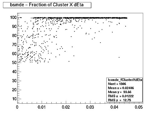
How to Use
In order to follow the same scheme done in StAssociationMaker we save the association information in multimaps. Multimaps make it very easy for the user to get the association information for a given StMcTrack, cluster or point. Detailed documentation for StAssociationMaker is available <a href="http://www.star.bnl.gov/STAR/comp/pkg/dev/StRoot/StAssociationMaker/doc/">here</a>. There are essentially four multimaps defined for the BEMC:- multiEmcTrackCluster - correlates the StMcTrack with StEmcClusters
- multiEmcClusterTrack - corrrelates the StEmcCluster with StMcTracks
- multiEmcTrackPoint - correlates the StMcTrack with StEmcPoints
- multiEmcPointTrack - correlates the StEmcPoint with StMcTracks
StEmcAssociationMaker *emcAssoc = GetMaker("EmcAssoc");
if(!emcAssoc) return;
multiEmcTrackCluster *map = emcAssoc->getTrackClusterMap(1);
if(!map) return;
for(multiEmcTrackClusterIter j=map->begin(); j!=map->end(); j++)
{
  StMcTrack* track = (StMcTrack*)(*j).first;
  StEmcClusterAssociation* value = (StEmcClusterAssociation*)(*j).second;
  if(track && value)
  {
    StEmcCluster *c = (StEmcCluster*) value->getCluster();
    if(c)
    {
      cout <<" McTrack = "<<track<<" GeantId = "<<track->geantId()
           <<" pt = "<<track->pt()<<" TReta = "<<track->pseudoRapidity()
           <<" Cl = "<<c<<" E = "<<c->energy()<<" eta = "<<c->eta()
           <<" phi = "<<c->phi()
           <<" FrTr = "<<value->getFractionTrack()
           <<" FrCl = "<<value->getFractionCluster()<<endl;
    }
  }
} Makers
The BEMC makers available in STAR include:
StEmcADCtoEMaker - This maker converts plain ADC values in energy. It subtracts pedestals, applies calibrations and creates the StEmcRawHits in StEvent. This maker also checks for corrupted headers. The input data format for this maker can be ANY of the formats below:
- DAQ format (from DAQ files)
- StEmcRawData format (StEvent)
- StEmcCollection (StEvent)
- StMuEmcCollection (muDST)
A light version of this maker (StEmcRawMaker) runs during production. StEmcRawMaker uses only DAQ or StEmcRawData format as input.
StPreEclMaker - This maker implements clustering of the BEMC detectors.
StEpcMaker - This maker matches the clusters in the BEMC detectors making what we call an StEmcPoint. It also matches tracks with points, if the input format is StEvent.
StEmcTriggerMaker - This maker simulates the BEMC level 0 trigger response using the plain ADC information from the towers. It works both with real and simulated data and it applies exactly the same trigger algorithm as in the BEMC hardware.
StEmcSimulatorMaker - This is the slow BEMC simulator. It takes an StMcEvent as input and fills the StEmcRawHit collections of StEvent with simulated ADC responses for all subdetectors.
StEmcCalibrationMaker - This is the maker used for BEMC calibration. It has methods to calculate pedestals for all the BEMC detectors as well as detector equalization, based on spectra shape and MIP analysis. This maker runs online as our online pedestal calculator.
StEmcMixerMaker - This maker is the basic BEMC embedding maker. It mixes hits from two StEvent objects in the memory. The hits from the second StEvent are mixed in the first one. It can run in a standard BFC embedding chain or as an afterburner (afterburner mode requires an event.root file from non-BEMC embedding plus a geant.root file containing BEMC information for simulated particles to be embedded).
StEmcTriggerMaker
Documentation provided by Renee FatemiMOTIVATION:
- Apply online trigger algorithm to simulated data
- Apply "software trigger" to triggered data
- Ensure that the same code is used for case 1. and 2.
How the Code Works:
StEmcTriggerMaker is the class that provides the user access functions to the trigger decisions. The workhorse is the StBemcTrigger class. StEmcTriggerMaker passes a StEvent pointer from either StEmcADCtoEMaker (real data) or StEmcSimulatorMaker (simulated data). The code accesses all offline status/ped/calibrations from StBemcTables, which are set in the macro used to run the code (ideal status/gain/ped can also be set). Code uses StEmcCollection to access ADC for all WEST BEMC channels which are not masked out with the status code and perform FPGA+L0 trigger on 12 bit ADC and 12 bit PED.
Access Function Examples:
    //  if event fulfills trigger return 1 else return 0  problems return -1
    int            is2005HT1() {return mIs2005HT1;}
    int            is2005JP1() {return mIs2005JP1;}

    // The ID of  the candidate HT (JP)
    int            get2005HT1_ID() {return HT1_ID_2005;}
    int            get2005JP1_ID() {return JP1_ID_2005;}

    // The DSM ADC of the candidate HT (JP)
    int            get2005HT1_ADC() {return HT1_DSM_2005;}
    int            get2005JP1_ADC() {return JP1_DSM_2005;}

    //  The number of towers(patches) and the id’s which fulfill the trigger
    void           get2005HT1_TOWS(int, int*);//array of tow ids passing HT1_2005 trig
    int             get2005HT1_NTOWS() {return numHT1_2005;}//# tows passing HT1_2005 trig
    void           get2005JP1_PATCHES(int, int*);//array of patches passing JP1_2005
    int             get2005JP1_NPATCHES() {return numJP1_2005;}//# patches passing JP1_2005
These access functions exist for 2003 HT1, 2004 HT1+JP1, 2005 HT1+HT2+JP1+JP2
CODE EXAMPLE:
   //get trigger info
    trgMaker=(StEmcTriggerMaker*)GetMaker("StEmcTriggerMaker");
    HT1_2005_evt=-1;
    HT1_2005_id=-1;
    HT1_2005_dsm=-1;
    numHT1_2005=0;
    HT1_2005_evt=trgMaker->is2005HT1();
    HT1_2005_id=trgMaker->get2005HT1_ID();
    HT1_2005_dsm=trgMaker->get2005HT1_ADC();
    numHT1_2005=trgMaker->get2005HT1_NTOWS();
    for (int i=0;i<numHT1_2005;i++){
      int towerid=-1;
      trgMaker->get2005HT1_TOWS(i,&towerid);
      HT1_2005_array[i]=towerid;
    }
COMMENTs for DISCUSSION:
Conceptually this code was designed from a software/analysis user point of view. Consequently I do not explicitly calculate and store all levels of DSM logic (it is unnecessary). From my understanding this is precisely what the StEmcTriggerDetector class was written to do -- return all DSM levels. It propagates all of the trigger information to the MuDst. BUT the problem is that this class is not propagated to the simulation (as far as I can tell). Even if it was propagated we probably wouldn’t want to take this option because it limits the usefulness of the simulation, whereas the StEmcTriggerMaker allows flexibility in applying the trigger algo to any simulation set. It is certainly possible code up the 2006 part of StEmcTriggerMaker to return all BEMC and EEMC trigger patch information at all levels of DSM, but it doesn’t exist in the current code.
Utilities
These are not Makers but codes that prove useful for BEMC analyses. The headings indicate where the codes can be found in the STAR source code repository.
StRoot/StDaqLib
EMC/StEmcDecoder
This utility converts the daq indexes for any BEMC detector (crate number, position in the crate, etc) in software ids (softId, module, eta, sub).
It also converts the Level-0 BEMC trigger patches ids in the corresponding tower crate number and index in the crate. It is quite useful to determine the correspondent tower that fired the trigger
StRoot/StEmcUtil
geometry/StEmcGeom
This class is used to convert softId in real eta and phi position in the detector and vice-versa. Also converts softId in module, eta and sub indexes that are used in StEvent.
It has methods to get geometrical information of the BEMC, such as number of channels, radius, etc. This is a very important utility in the BEMC software.
projection/StEmcPosition
Utility to project tracks in the BEMC detector
database/StBemcTables
Utility to load the database tables and get any information from them. It works only in makers running in the chain and has methods to return pedestal, calibrations, gain and status values for all the BEMC detectors. To use it do, in your maker:
// in the constructor. Supposing you have a private
// member StBemcTables *mTables;
mTables = new StBemcTables();
// in the InitRun() or Make() method
// this method loads all the BEMC tables
// it is necessary to have St_db_Maker running
mTables->loadTables((StMaker*)this);
// Getting information
// for example, getting pedestal and RMS for the
// BTOW Detector softId = 100
float ped = mTables->pedestal(BTOW, 100);
float rms = mTables->pedestalRMS(BTOW, 100);
database/StBemcTablesWriter
This class inherits from StBemcTables and is useful for performing all kinds of more advanced BEMC DB operations, including uploading tables if you've got the privileges for it.
I'm not sure if anyone is actually using the rest of these, nor am I confident that they actually work in DEV. Feel free to leave some feedback if you have some experience with them. -- Adam
hadBackground/StEmcEnergy
Utility to subtract hadronic energy from EMC towers. It uses StEmcHadDE to subtract the hadronic energy in the calorimeter in a event by event basis.
hadBackground/StEmcHadDE
Utility to calculate hadronic energy profile in the BEMC. It calculates the amount of energy deposited by a single hadron as a function of its momentum, position in the detector and distance to the center of the tower.
voltageCalib/VoltCalibrator
This utility calculates high voltages for the towers for a given absolute gain.
neuralNet/StEmcNeuralNet
Basic EMC neural network interface.
filters/StEmcFilter
Event filter for BEMC (StEvent and StMcEvent only)
This utility has a collection of tools to do event filtering in the BEMC. Some of the filters available are:
- basic event filter: vertex, multiplicity, etc
- tower filters: tower isolation filter, number of tracks in tower, energy cuts, tower energy and associated pt cuts, etc.
Useful Documents
A full list of attached documents is available below, but I wanted to highlight a few here:
BEMC Technical Design Report (PDF)
Run 9 BSMD Online Monitoring Documentation
For run 9, BSMD performance was monitored by looking at non-zero-suppressed events. The code is archived at /star/institutions/mit/wleight/archive/bsmdMonitoring2009/. This blog page will focus on the details of how to run the monitoring and the importance of various pieces of code involved in the monitoring. The actual monitoring plots produced are discussed here.
A few general notes to begin:
Since the code all sat in the same directory constantly, a number of directories have been hard-coded in. Please make sure to change these if necessary.
The code for actually reading in events is directly dependent on the RTS daq-reader structure: therefore it sits in StRoot/RTS/src/RTS_EXAMPLE/.
All compilation is done using makefiles.
Brief Description of the Codes:
This section lists all the pieces of code used and adds a one- or two-sentence description. Below is a description of the program flow which shows how everything fits together. Any other code files present are obsolete.
In the main folder:
runOnlineBsmdPSQA.py: The central script that runs everything.
onlBsmdPlotter.cxx and .h: The code that generates the actual monitoring plots. To add new plots, create a new method and call it from the doQA method.
makeOnlBsmdPlots.C: Runs the onlBsmdPlotter code.
GetNewPedestalRun.C: Finds the newest BSMD pedestal run by querying the database.
onlBsmdMonConstants.h: Contains some useful constants.
cleanDir.py: Deletes surplus files (postscript files that have been combined into pdfs, for instance). This script is NOT run by runOnlineBsmdPSQA.py and must be run seperately.
In the folder StRoot/RTS/src/RTS_EXAMPLE/
bsmdPedMonitor.C: Reads the pedestal file from evp and fills and saves to file the pedestal histograms, as well as generating ps and txt files describing the pedestals.
makeMapping.C: Creates a histogram that contains the mapping from fiber and rdo to softId and saves it to mapping.root. Unless the mapping changes or the file mapping.root is lost there is no need to run this macro.
onlBsmdMonitor.C: Reads BSMD non-zero-suppressed events as they arrive and creates a readBarrelNT object to fill histograms of pedestal-subtracted ADC vs. softId and capId, as well as rates and the number of zero-suppressed events per module. When the run ends, it saves the histograms to file and quits.
readBarrelNT.C and .h: This class does the actual work of filling the histograms: used by onlBsmdMonitor.C.
testBsmdStatus.C: Checks the quality of the most recent pedestal run and generates QA ps files.
rts_example.C: This is not used but serves as the template for all the daq-reading code.
Program Flow:
The central script, runOnlineBsmdPSQA.py, has a number of options when it is started:
Script Options
-p: print. This is a debugging option: it causes the code to print the ADC value for every channel.
-n: number of events (per run). Occasionally it is useful to limit the number of (non-zero-suppressed) events the monitoring program looks at for tests. During actual monitoring, we wished to catch all possible events so the script was always initialized with -n 1000000: the actual number of non-zero-suppressed events in a run is a few hundred at most.
-t: this option is not used in the current version of the code.
-r: raw data. This option was added during testing when online reading of pedestal files had not been implemented: if it is turned on then the code will not attempt to subtract pedestals from the data it reads.
-v: mpv cut. If a channel has MPV greater than this value, it is considered to have a bad MPV. The default is 5.
-m: mountpoint. For monitoring, the mounpoint is always set to /evp/. During tests, it may be useful not to have a mountpoint and read from a file instead, in which case no mountpoint will be given.
The standard initialization of the script for monitoring is then:
python runOnlineBsmdPSQA.py -n 1000000 -m /evp/
Usually the output is then piped to a log file. For testing purposes, as noted above, the -m option can be left off and the mountpoint replaced with a file name. (Side note: if neither a mountpoint nor a file name is given, the code will look for the newest file in the directory /ldaphome/onlmon/bsmd2009/daqData/, checking to be sure that the file does not have the same run number as that of the last processed run. This last option was implemented to allow for continuous processing of daq files but never actually used.)
The main body of the monitoring script is an infinite loop. This loop checks first to see what the current BSMD pedestal run is: if it is newer than the one currently used, the script processes it to produce the pedestal histograms that will be used by the data processing code. This process happens in several steps:
Pedestal Processing
Step 1: The script calls the C macro GetNewPedestalRun.C, passing it the time in Unix time format. The macro then queries the database for all pedestal runs over the last week. Starting with the most recent, it checks to see if the BSMD was present in the run: if so, the number of that run is written to the file newestPedRunNumber.txt and the macro quits.
Step 2: The script opens newestPedRunNumber.txt and reads the run number there. It then checks to see if the pedestals are up-to-date. If not, it moves to step 3.
Step 3: The script moves to StRoot/RTS/src/RTS_EXAMPLE/ and calls bsmdPedMonitor, passing it the evp location of the newest pedestal run, /evp/a/runnumber/ (bsmdPedMonitor does take a couple of options but those are never used). The main function of bsmdPedMonitor is to produce a root file containing three histograms (BSMDE, BSMDP, BPRS) each of which has a pedestal value for each softId-cap combination. The pedestal monitoring code starts by reading in the BSMD and BPRS status table (StatusTable.txt) and the mapping histogram (from the file mapping.root) which gives the mapping from fiber and rdo to softId. Then it goes into an infinite loop through the events in the file. In a pedestal file, the pedestals are stored in the event with token 0: therefore the code rejects events with non-zero token. Once it has the token-0 event, it loops through the fibers, grabs the pedestal and rms databanks for each fiber, and fills its histograms. Finally the code generates a text file that lists every pedestal and several ps files containing the pedestals plotted vs softId and cap.
Step 4: The script calls testPedStatus.C, passing it the root file just generated. This macro checks for each good channel to make sure that the pedestals and rms just obtained are within certain (hardcoded) limits. If the number of channels that have pedestal or rms outside of these limits is above a (hardcoded) threshold for a given crate, that crate is marked as bad. A ps file is generated containing a table in which crates are marked as good or bad with green or red and several more with softId vs cap histograms in which bad pedestals are marked in red.
Step 5: The postscript files are combined into pdfs (one for the pedestals and one for the statuses), which are, along with the text file, copied to the monitoring webpage. The index.html file for the monitoring webpage is updated to reflect that there are new pedestals and to link to the files generated from the new pedestal file. Finally, the variable containing the number of the old pedestal run is changed to that of the current pedestal run.
The next step is to call onlBsmdMonitor, which reads the events as they arrive. This code has several options:
Daq Reading Options:
-d: allows you to change the buillt-in rts log level.
-D: turns on or off printing: corresponds to -p from the script.
-m: mountpoint, the same as -m from the script.
-n: nevents, the same as -n from the script.
-l: last run, which tells the code what the last run was so that it knows when a new run is starting.
-r: raw data, same as -r from the script.
The script thus picks what options to give to onlBsmdMonitor from the options it was given, as well as from the value it has recorded for the last run number (1 if the script is starting up). Output from onlBsmdMonitor is piped to a log file named currentrun.log. OnlBsmdMonitor also consists of an infinite loop. As the loop starts, it gets the current event, checks to see if we are in a new run, and if so that this new run has the BSMD in. If so, it initializes a new instance of the class readBarrelNT, which does the actual processing, and then processes the event. If instead this is an already-occuring run, it checks to make sure that we have a new event, and if so processes it. If we are in between runs or the event is not new, the loop is simply restarted, in some cases after a slight delay. The main task of onlBsmdMonitor is to obtain histograms of pedestal-subtracted ADC vs softId and capId for the BPRS, BSMDE, and BSMDP and save them to a root file. It also histograms the rate at which events are arriving and the number of zero-suppressed events per module. The root file also contains a status histogram which is obtained from file StatusTable.txt. When the run is over, the histograms are written to file and onlBsmdMonitor quits, writing out a line to its log file to indicate its status at the point at which it ends.
The script now looks at the last line of the log file. If this line indicates that the run had no BSMD, a new entry in the monitoring webpag's table is created to reflect this fact. If not, the script first checks to see if we are in a new day: if so, a new line for this day is added to the webpage and a new table is started. The script then extracts the number of non-zero-suppressed BSMD events, the total number of events in the run, the number of ZS events, and the duration of the run from the last line of the log file. If the run is shorter than a (hardcoded) length cutoff, has no NZS BSMD events, or has fewer NZS BSMD events then a (hardcoded) threshold, the appropriate new line in the table is created, with each of the values obtained from the log file entered into the table, a link to the runlog added, and the problem with the run noted. If the run passes all quality checks, makeOnlBsmdPlots is called. This code generates the actual monitoring plots: the script then takes the resulting ps files, combines them into a pdf, and creates a new entry in the table with all the run information, a link to the pdf, a link to the run log, and a link to pedestal QA pdf. The plotting code requires to be given the mpv cut value and the elapsed time, as well as the name of the root file containing the histogram for the runs. Any new monitoring plots that are desired can be added by adding a method to create them to onlBsmdPlotter.h and onlBsmdPlotter.cxx and calling them in the method doQA. Having thus completed a run, the loop restarts.
Some BSMD hardware documents
Some BSMD hardware documents, below