Efficiency of reconstructing photons in EEMC

Monte Carlo sample

• 10k photons
• STAR y2006 geometry
• z-vertex=0
• Flat in pt 10-30 GeV
• Flat in eta 1.0-2.1

SMD gamma/pi0 discrimination algorithm

The following

slide

from the IUCF STAR Web site gives a brief overview of the SMD gamma/pi0 discrimination algorithm using the method of maximal sided fit residual (data - fit). This technique comes to STAR EEMC from the Tevatron via Les Bland via Jason Webb. The specific fit function used in this analysis is:

f(x)=[0]*(0.69*exp(-0.5*((x-[1])/0.87)**2)/(sqrt(2*pi)*0.87)+0.31*exp(-0.5*((x-[1])/3.3)**2)/(sqrt(2*pi)*3.3))

x is the strip id in the SMD-u or SMD-v plane. The widths of the narrow and wide Gaussians are determined from empirical fits of shower shape response in the EEMC from simulation.

Optimizing cuts for gamma/pi0 separation

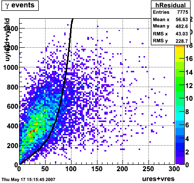
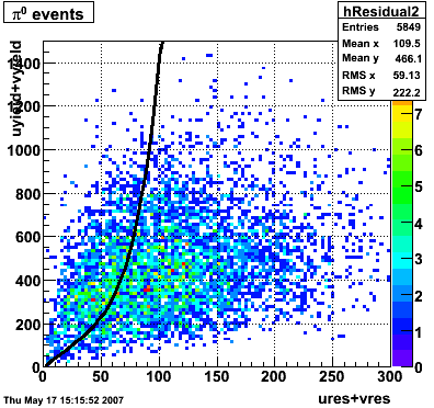
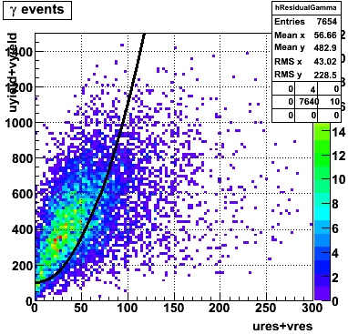
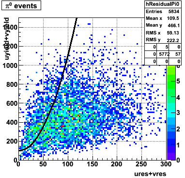
In the rest of this analysis, only those photons which have reconstructed pt > 5 GeV are kept. There is no requirement that the photon doesn't convert. The dividing curve between photons and pions is:

f(x)=4*x+1e-7*x**5

The y-axis is integrated yield over the SMD-u and SMD-v plane, and the x-axis is the sum of the maximal sided residual of the SMD-u and SMD-v plane.

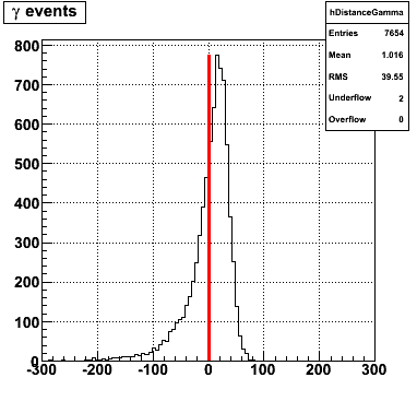
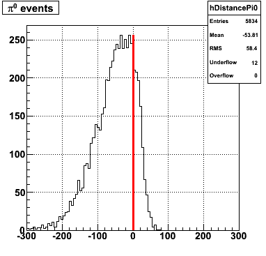
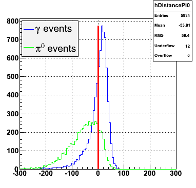
Following exchanges with Scott Wissink, the idea is to move from a quintic to a quadratic to reduce the number of parameters. In addition, the perpendicular distance between the curve and a point in the plane is used to estimate the likelihood of a particle being a photon or pion. Distances above the curve are positive and those below are negative. The more positive the distance, the more likely the particle is a photon. The more negative the distance, the more likely the particle is a pion.

Hi Pibero,

With your new "linear plus quintic" curve (!) ... how did you choose the
coefficients for each term?  Or even the form of the curve?  I'm not
being picky, but how to optimize such curves will be an important issue
as we (hopefully soon) move on to quantitative comparisons of efficiency
vs purity.

As a teaser, please see attached - small loss of efficiency, larger gain
in purity.

Scott

Hi Pibero,

I just worked out the distance of closest approach to a curve of the form

    y(x) = a + bx^2

and it involves solving a cubic equation - so maybe not so trivial after
all.  But if you want to pursue this (not sure it is your highest
priority right now!), the cubic could be solved numerically and "alpha"
could be easily calculated.

More fun and games.

Scott

Hi Pibero,

I played around with the equations a bit more, and I worked out an
analytic solution.  But a numerical solution may still be better, since
it allows more flexibility in the algebraic form of the 'boundary' line
between photons and pions.

Here's the basic idea:  suppose the curved line that cuts between
photons and pions can be expressed as y = f(x).  If we are now given a
point (x0,y0) in the plane, our goal is to find the shortest distance to
this line.  We can call this distance d (I think on your blackboard we
called it alpha).

To find the shortest distance, we need a straight line that passes
through (x0,y0) and is also perpendicular to the curve f(x).  Let's
define the point where this straight line intersects the curve as
(x1,y1).  This means (comparing slopes)

    (y1 - y0) / (x1 - x0) = -1 / f'(x1)

where f'(x1) is the derivative of f(x) evaluated at the point (x1,y1). 
Rearranging this, and using y1 = f(x1), yields the general result

    f(x1) f'(x1)  -  y0 f'(x1)  +   x1  -   x0  =  0

So, given f(x) and the point (x0,y0), the above is an equation in only
x1.  Solve for x1, use y1 = f(x1), and then the distance d of interest
is given by

    d = sqrt[ (x1 - x0)^2 + (y1 - y0)^2 ]

Example:  suppose we got a reasonable separation of photons and pions
using a curve of the form

    y = f(x) = a + bx^2

Using this in the above general equation yields the cubic equation

    (2b^2) x1^3  +  (2ab + 1 - 2by0) x1  -  x0  =  0

Dividing through by 2b^2, we have an equation of the form

    x^3 + px + q = 0

This can actually be solved analytically - but as I mentioned, a
numerical approach gives us more flexibility to try other forms for the
curve, so this may be the way to go.  I think (haven't proved
rigorously) that for positive values of the constants a, b, x0, and y0,
the cubic will yield three real solutions for x1, but only one will have
x1 > 0, which is the solution of interest.

Anyway, it has been an interesting intellectual exercise!

Scott

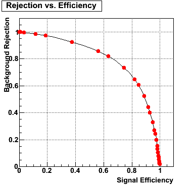
I made use of the ROOT function TMath::RootsCubic to solve the cubic equation numerically for computing distances of each point to the curve. With the new quadratic curve f(x)=100+0.1*x^2 the efficiency is 63% and the rejection is 82%.

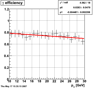
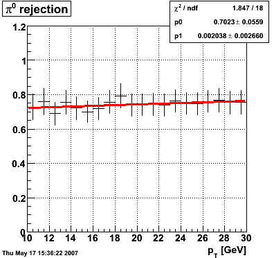
Efficiency and Rejection

The plot on the left below shows the efficiency of identifying photons over the pt range of 10-30 GeV and the one on the right shows the rejection rate of single neutral pions. Both average about 75% over the pt range of interest.

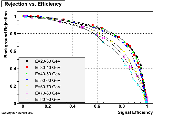
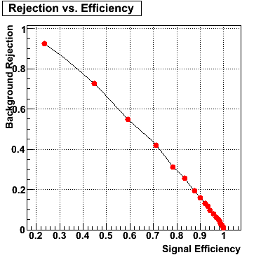
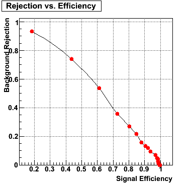
Rejection vs. efficiency at different energies

The plot below shows background rejection vs. signal efficiency for different energy ranges of the thrown gamma/pi0.

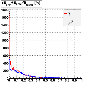
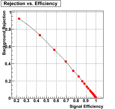
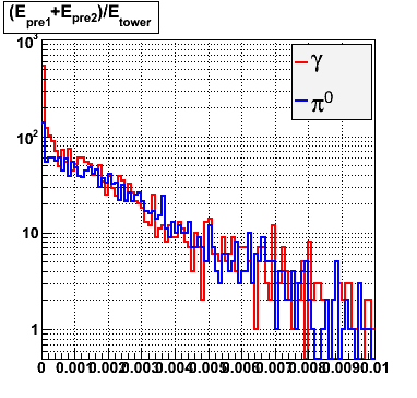
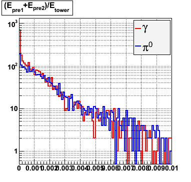
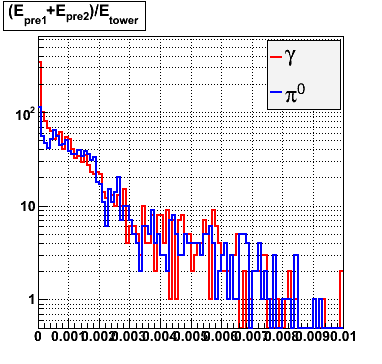
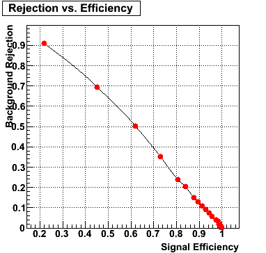
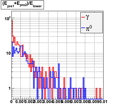
Rejection vs. efficiency with preshower cut

Below on the left is a plot of the ratio of the sum of preshower 1 and 2 to tower energy for both photons (red) and pions (blue). On the right is the rejection of pions vs. efficiency of photons as I cut on the ratio of preshower to tower. It is clear from these plots that the preshower layer is not a good gamma/pi0 discriminator, although can be used to add marginal improvement to the separation preovided by the shower max.

ALL ENERGIES
E=20-40 GeV
E=40-60 GeV
E=60-80 GeV
E=80-90 GeV